Time domain signal descriptors

Frequency vs time domain

Description and classification of audio signals such as music or speech often relies on frequency domain techniques, because the processing in the inner ear is somewhat similar to a transformation from the time domain to the frequency domain. We are not good at detecting phase differences between two sounds with identical amplitude spectrum, even though their waveforms look very different.

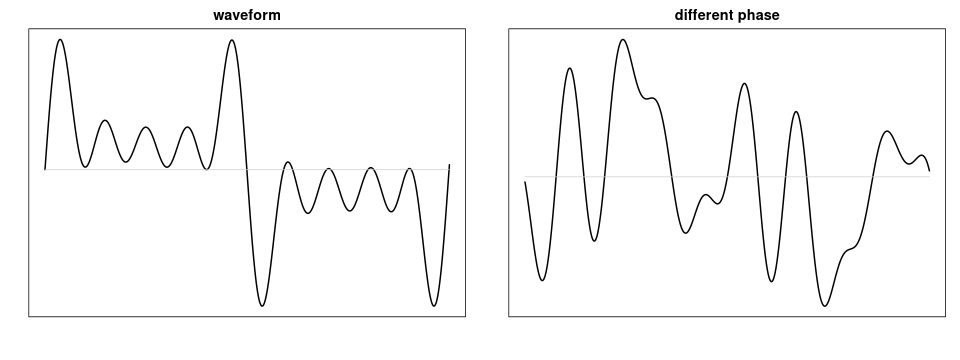
Two waveforms with identical amplitude spectrum and partials in different phases

Corresponding amplitude spectrum

Feature extraction of audio signals is therefore often carried out in the frequency domain using an FFT or other transforms, but some features can be retrieved in the time domain. The term feature extraction has connotations of something that corresponds to perceivable traits in the sound, such as loudness or pitch on a fundamental level, or rhythmic and tonal attributes such as tempo and key on a higher level. Signal descriptors are more modest in ambition and characterise some measurable quantities in signals without necessarily indicating what audible attribute they relate to.

In musical audio, signal descriptors find use in Music Information Retrieval (MIR), adaptive effects, adaptive synthesis, and sound analysis for various purposes such as segmentation and source classification. Signal descriptors also have applications in areas such as speech recognition, environmental monitoring, medical diagnostics, and machine failure detection.

For some researchers, a goal of machine listening, as it is often called, is to mimic human capabilities. Among the ultimate consequences, whether intended or not, is to render the human capability second rate and possible to automate away.

Ideally, we would like machines and computers to be aware of their immediate surroundings as human beings are. [...] Therefore, in the quest for making computers sense their environment in a human-like way, sensing the acoustic environment in broad sense is a key task. (Alías et al., 2016)

Or, in the words of another group of authors:

Ideally, in today’s world we want computers to have capability to make decisions like humans. One of the important sense of humans is hearing. [...] We want machines would be able to classify between various sounds as humans can do effortlessly. (Sharma et al., 2019)

Ideally, one may add, we would want AI to be able to render each and everyone superfluous in our capacity as creative beings. At least until it actually happens. There are many reasons to be critical of naïve techno optimism, which is not to say that all technology must be rejected. Another point, particularly relevant to feature extraction, is the trend toward computationally complex models. A certain complexity is necessary even to remotely mimick human auditory abilities, but one of the motivations for the set of signal descriptors introduced here is to keep it simple, small, and efficient.

Frequency domain techniques based on the Short-Time Fourier Transform have been prevalent in MIR and other musical applications, and more recently they have been complemented by other signal representations such as cepstrum, wavelet transforms, or treating the spectrogram as a 2D image. Still, some elementary time domain descriptors can be a useful complement. The spectral centroid and some other descriptors have an obvious definition in the frequency domain, but can be implemented in the time domain as well. In fact, the principle of time-frequency duality relates some operations performed in one domain to its dual in the other domain, such as multiplication and convolution. Many operations are easily handled in one of the domains and non-trivial or impossible in the other. If there is a paucity of time domain signal descriptors, the reason might be the closer correspondence of spectral features to audio perception, but perhaps there has also been a lack of imagination. To break with that trend, we introduce a few novel time domain signal descriptors among some old ones.

However, not all time domain descriptors found in the MIR literature are presented here. One notable omission concerns those that describe features of an already segmented sound, such as log attack time and temporal centroid.

A collection of signal descriptors

The implementation of the following signal descriptors is simple and efficient, and follows a similar pattern. Specifically, they receive an input signal $x_n$ one sample at a time and return an output signal $\phi_n$ at the same sample rate. Internally, there is a sliding analysis window, which means that each output value is a function of the input signal's recent history, $\phi_n = f(x_n, x_{n-1}, x_{n-2}, \ldots).$ There is a loss of information and, usually, some redundancy in the output signal. For analysis purposes, one may throw away most output samples and display as little as two to four from each time window.

None of the descriptors take notice of the input signal's sampling rate. Some values may change significantly if they are passed an upsampled or downsampled version of the same signal.

Buffered processing is an option when performance is a priority; that is, instead of calling the function once for each sample one calls it with an array of several samples. In principle, these algorithms always deliver one output sample for each input sample. Using buffering introduces a latency, which makes a significant difference if the signal descriptor is inside of a feedback loop, or a feature extractor feedback system (FEFS), as I have used to called them. In feedback scenarios the function should be called once for each sample.

RMS amplitude

Measuring the local amplitude over a short signal segment is a basic operation that is needed in many other descriptors. There are a few ways to do this. To measure the amplitude over a sliding rectangular window of length L, the formula is: $$ u_n = x_{n}^{2} / L $$ $$ v_n = v_{n-1} + u_n - u_{n-L} $$ $$ rms(x_n) = \sqrt{v_n} $$ An efficient implementation uses a circular buffer for $u_n$. This structure is known as TIIR, or truncated infinite impulse response, which is a clever way of making a recursive filter have a finite impulse response.

Another implementation uses a leaky integrator, which is a one-pole lowpass filter with very low cutoff frequency. In most cases, the descriptors operate on an equally weighted chunk of consecutive samples, which is sometimes called a box-car filter. If a leaky integrator is used, its infinite impulse response means that the effective window size is not clearly defined, but for practical purposes it can be taken to be the time after which the impulse response has dropped by some amount, say, -24 dB.

Instead of squaring the input signal, one might use the full-wave rectifier $u_n = |x_n|$ or half-wave rectifier $u_n = \max(0,x_n),$ in which case the square root is omitted.

Simple loudness estimation can be achieved by pre-filtering the signal such that frequencies in the most sensitive range of hearing, around 3-4 kHz, are emphasised, whereas low and very high frequencies are rolled off.

Peak-to-peak amplitude and asymmetry

Another amplitude measure, more common in electronics, is the peak-to-peak amplitude, $pp_n = \max(x_{n}) - \min(x_{n})$, where the maximum and minimum are sought within the current time window. A more practical approach for a sliding descriptor is to compare the current sample to stored min and max variables, and if the current sample overshoots them, their value is replaced by the current sample. But the current extreme values also need to be forgotten somehow. We do this by introducing a decay; the min and max are multiplied by a coefficient $g<1$ close to one.


if(x > max)
	max = x;
if(x < min)
	min = x;

pp = (max-min)/2;
max *= g;
min *= g;

The full amplitude range of a signal that varies in the interval [-1,1] would be 2, but for the sake of direct comparability with other amplitude measures it is divided by two.

Asymmetry in the vertical direction, or the difference between the heights of positive and negative peaks, is obtained simply by reversing a sign: $a_n = max_n + min_n$ (division by 2 is omitted). There doesn't have to be a DC-offset for a signal to have significant vertical asymmetry. Sharply peaking signals may have a high positive peak and spend most time at small negative values, and may still average to zero over a period.

Centroid

Using an FFT, the spectral centroid is calculated from the amplitude spectrum with bins $a_k$ as $$ C_n = \frac{\sum k a_k}{\sum a_k} $$ in units of frequency bins. The multiplication by k emphasises high frequencies; in fact, it corresponds to differentiation in the time domain. Therefore, the centroid can be estimated using a differentiating filter (which we write as $\Delta$) and two rms units as follows: $$ c_n = \frac{rms(\Delta x_n)}{rms(x_n)}. $$ The differentiator is a FIR filter with impulse response $ \{ \ldots, -1/3, -1/2, -1, 0, 1, 1/2, 1/3, \ldots \}$ centred at 0. A simple differentiator with impulse response $\{1,-1\}$ is often used, but including more coefficients improves the estimate of the centroid. However, the frequency response of these improved differentiating filters actually has a zero at the Nyquist frequency. For practical purposes, this is not a serious drawback unless it is important to detect such high frequencies.

Spectral flux

The amount of change in the amplitude spectrum from one analysis window to the next is measured by the spectral flux. A time domain version can be built from a filter bank of bandpass filters and rms measurements at the current time as compared to a delayed time.

Using spectral flux, one should be able to identify pitch changes between analysis windows, even though the amplitude remains constant. Spectral flux also spots note onsets and endings particularly well.

As proof of concept, a minimalist spectral flux detector might use just a highpass and a lowpass filter realised as one zero filters, two delays, and two RMS amplitude detectors. The spectral flux is measured as the difference in amplitude in the two frequency bands at lag L, which is the same as the effective length of the RMS detectors.

$$ a_{lo,n} = RMS(x_n + x_{n-1}) $$ $$ a_{hi,n} = RMS(x_n - x_{n-1}) $$ $$ \Phi_n = \frac{1}{2}(|a_{lo,n} - a_{lo,n-L}|)+ |a_{hi,n} - a_{hi,n-L}| )$$

Perhaps it is an exaggeration to call this a spectral flux descriptor, but it does capture transients such as onsets and endings very well. Without much loss, it might be simplified further by taking the difference, without filtering, between the current and delayed rms amplitude of the input signal.

Zero crossing rate

In a monodic signal with constant waveform, the number of zero crossings per time unit is proportional to the fundamental frequency. Similar to the centroid, it is also related to the amount of high frequency content.

The basic implementation idea is best described in pseudo code. When a zero crossing occurs, a counter is incremented and the boolean variable flag is set to true; then, if this flag was true L samples ago, which means there was a zero crossing at that point, the counter is decremented by one, and the zcr is the counter divided by the lag.


flag[n] = false; 
if( x[n]*x[n-1] < 0 ) // a zero crossing occurs 
	{
	++count; 
	flag[n] = true;	
	}
if(flag[n-L])	// actually needs a delay of the flag variable
	--count;	

zcr = count / L;

Zero crossing rate over a fixed time window suffers from the familiar time/frequency resolution problem: poor frequency resolution at low frequencies or poor time resolution at high frequencies. There is an alternative way to measure zcr – adaptively over a variable window length. The time T it takes for the signal to do M zero crossings is counted. Then, we simply have zcr = M/T, a value that is updated each time there is a zero crossing.

Robustness against background noise may sometimes be desirable. It is achieved by setting a small threshold above and below 0 that the signal must cross for the zero crossing to count.

Total variation

In real analysis math books one encounters a concept known as total variation. Simply put, it measures the distance travelled on the graph of a one-dimensional function, which is why it is also sometimes refered to as waveform length. As we consider discrete time signals, all the intricacies of real analysis fortunately vanish. The total variation, measured locally over the last L samples, is the sum of differences between adjacent samples, and to make it independent of the window length we normalise by dividing by L. $$ tv_n = \frac {1}{2L} \sum_{k=0}^{L-1} |x_{n-k} - x_{n-1-k}| $$

The total variation increases with both amplitude and frequency. At the Nyquist frequency and a signal with peak amplitude 1, its value reaches the theoretical maximum of 1. Such signals are rare in musical audio, typical values are closer to zero. A centroid-like descriptor can be derived by dividing the total variation by the amplitude over the same window length.

Extrema

Similar to zero crossings, the average distance between waveform peaks is a useful measure which correlates with frequency. Since there is always one negative peak somewhere between two positive peaks one doesn't lose much information by counting only positive (or only negative) peaks, except that the temporal accuracy is better if both are taken into account.

The distribution of the latest few inter-peak spacings can be further analysed. Perfectly regular waveforms at a fixed frequency, with exactly one peak per cycle, have a spike distribution, all peak distances being the same. Tones with prominent formants may have several peaks per cycle with different distances between them. Chords, inharmonic sounds, and noisy sounds have increasingly irregular peak intervals. Useful statistics are the standard deviation and entropy of the distribution. The minimum peak distance gives an indication of the period corresponding to the highest prominent partial.

Power difference

The idea is to take the average difference of the power $x_{n}^2$, and normalise with respect to the average power over the last L samples. This amounts to applying the time domain version of the centroid to the squared signal, $$ \delta_n = |x_{n}^2 - x_{n-1}^2| $$ $$ powdif_n = \frac{\sum_k \delta_{n-k}}{\sum_k x_{n-k}^2} $$ where the sum runs from $k=0$ to $L-1$. This descriptor responds in particular to sharp onsets after silence and signals altering between full amplitude and zero every other sample.

Asymmetry

Time asymmetry, according to Kantz & Schreiber, is "a strong signature of nonlinearity" and may be an indication of some causal mechanism behind the time series. They also describe it as a higher-order autocorrelation. It is the running time average of a polynomial in $x_n$ and $x_{n-1}$ over some suitable window length.

$$ nlasym = \langle x_n x_{n-1}^2 - x_{n}^2 x_{n-1} \rangle $$

Using delayed variables, this can be calculated with just three multiplications, and one more to normalise the sum in the time average. This asymmetry measure is well able to distinguish between a chaotic signal from a discrete time dynamical system and random white noise, even though both signals have a flat amplitude spectrum.

Rising-to-falling ratio

Asymmetrical waveforms such as sawtooth or ramp spend most of their time rising (or falling), and reversing the waveform doesn't produce an audible difference under normal conditions. Still, the proportion of time the waveform rises versus falls can differentiate between many audibly different waveforms, such as triangle (equal time) versus ramp (only rising, except once per cycle).

The implementation resembles that of zcr, but is even simpler; the number of rising samples is counted and divided by the window size.

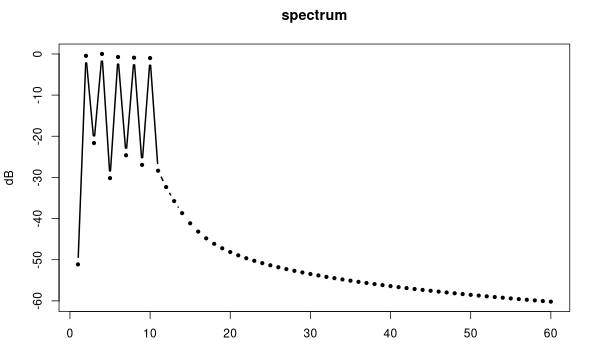
Waveform expansion

Yet another descriptor of the waveshape, expansion is defined as a consecutive pair of samples such that the next one is larger in absolute value.

$$ expand : |x_{n+1}| > |x_n| $$

Left: maximally expanding waveform; right: contracting or minimally expanding waveform.

The descriptor returns the proportion of expanding samples in the analysis window, thus its range is [0-1]. Symmetrical waveforms such as triangle, as well as sawtooth waveforms yield an expansion value of 0.5, which seems to be typical of most audio signals. A waveform ramping up from zero to 1, then snapping back to zero and ramping to -1, and snapping back to zero maximises expansion. Apart from perfect silence, it is minimised by waveforms with the opposite profile, that is, those that ramp towards zero, as well as square waves.

Convexity

We say that a signal is convex if it curves away from zero, either in the positive or negative direction. In a formula, whenever $$ |x_n| > |x_{n-1} + x_{n+1}|/2 $$ is true, the signal is convex. Equivalently, the second derivative of the absolute value is positive in a convex signal. Again, the descriptor returns the average convexity over the last samples.

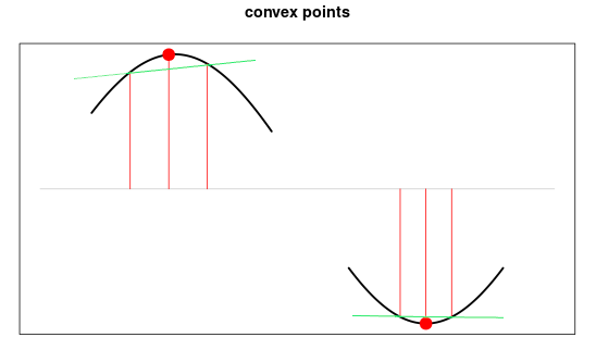
Convex points lie outside of the line joining their two adjacent samples.

Sinusoids and other smoothly curving waveforms maximise convexity, whereas straight line segments or cusp-shaped waveforms have minimal convexity.

Concavity

The opposite of convexity, this descriptor captures such things as exponentially decaying and cusp-shaped signals. Therefore it is also referred to as cusp. Let $p_n = |x_n|$. First we measure the overshoot $dy$ and count the number of times it is positive. $$ dy = (p_{n-1} + p_{n+1})/2 - p_n $$ $$ cusp_n = (\#(dy>0) + \sum dy) / L $$

In contrast to convexity, we also add to it the average overshoot.

Midband

The activity around $f_s/4$, or the middle of the spectrum, is contrasted to the activity in low and high bands. Two complementary second order FIR filters are used, with impulse responses $\{ 1,0,1 \}$ for a band reject profile that suppresses the middle frequency, and $\{ 1,0,-1 \}$ for a bandpass filter with zeros at DC and Nyquist. Absolute values are taken, and the bandpass output is divided by the notch.

$$ u = |x_n + x_{n-2}| $$ $$ v = |x_n - x_{n-2}| $$ $$ s = v/(u+1) $$ The quotient s then is time averaged.

Permutation entropy

An innovative technique proposed by Bandt & Pompe, the Permutation Entropy looks at contour types in sliding windows. A contour type is concerned with relative amplitude values, and how they are ordered. In a two point window the contour can be either rising or falling. A three point window has six contour permutations: (123), (132), (213), (231), (312), and (321). Bandt and Pompe did not treat ties (repeated values) as its own contour type, which we do in the present implementation. Also, only the patterns of rising or falling are taken into account, which leaves the five contour types, with R for rising and F for falling:

RR, RF, FR, FF, and "other" including ties.

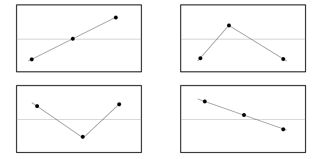
Four out of five contour types.

The rationale for treating ties as its own category is that perfect silence will then have its own contour type. Let $ p_i $ be the relative frequency of each of the five contour types. As usual, the relative frequency is taken over a sliding window. Then the Permutation Entropy is calculated as the Shannon entropy: $$ H = - \sum p_i \log p_i $$

A practical caveat: With three point permutation entropy, if the window slides one sample, the end of the previous contour will coincide with the beginning of the next contour. So, for instance, if the last direction in the previous contour was rising, the first direction in the next contour will also be rising. This introduces some redundancy and limits which contour types can follow any given contour type. In order to remove the redundancy the counting of contour types is skipped every other sample.

As the order or number of samples in the contour increases, the number of contour types grows, factorially in the original implementation, and exponentially in the present version. To keep it reasonably simple, in the spirit of the other descriptors in this collection, a three point permutation entropy is a good compromise. Each histogram bin for the five contour types requires its own delay line, which means that this descriptor uses five times the window length worth of memory space.

Shimmer

In voice quality assessments, shimmer is a measure of the amplitude variability between signal peaks where high variability may indicate some pathology. Naively, the distance between any nearest two positive peaks is measured. For a sinusoid or sawtooth wave it should be zero, but for waveforms with several peaks per cycle it would vary within each cycle. This can be overcome by looking for the maximum peak between two upwards zero crossings. When two adjacent peaks $p_0, p_1$ have been found, their amplitude difference $$ shimmer = |p_0 - p_1| $$ is the measure which, as usual, is averaged over an appropriate window length.

Slope sign change

The sign of the slope is +1 when the waveform is increasing and -1 when decreasing. A change of slope of course corresponds to a local maximum, either positive or negative. $$ SSC = \frac{1}{N} \sum_{n=0}^{N-1} f((x_n - x_{n-1})(x_n - x_{n+1}) ) $$ where $f(x) = 1$ for $x > \epsilon$ and $f(x) = 0$ otherwise, for some small positive threshold value $\epsilon.$ This descriptor can be generalised by counting changes of slope in certain intervals.

Autocorrelation

Lastly, a few other time domain descriptors deserve being mentioned even if they are not included in the source code.

Simple pitch followers use the autocorrelation function (acf). The first peak of the acf at a non-zero lag corresponds to the waveform's period, or the inverse frequency. In practice, the acf is preferably implemented using a discrete Fourier transform. If only one or a few specific lags are of interest, it can be done efficiently in the time domain.

Instantaneous amplitude and frequency

The Hilbert transform has interesting applications including frequency shifting. It takes a real valued signal $x_n$ and turns it into the complex valued analytical signal $z_n = x_n + iy_n$, where $y_n$ is a 90 degrees phase shifted version of $x_n$. It is often used to estimate the amplitude envelope $$ a_n = \sqrt{x_{n}^2 + y_{n}^2} $$ or the instantaneous frequency $$ f_n = \frac{f_s}{2\pi(x_{n}^2 + y_{n}^2)}(x_n\Delta y_n - y_n \Delta x_n) $$ where $f_s$ is the sampling frequency, and $\Delta$ is an approximation of the derivative (see Centroid, above). The instantaneous amplitude and frequency track fast changes in the signal, and may need to be smoothed.

Test signals

To get an idea of what the signal descriptors capture, we analyse a test signal consisting of segments of various types: Pink noise; white noise; a linear chirp from 12 kHz to 20 Hz; a pulse or DC-offset; an exponential decay; a 20 Hz sinusoid; a sine at $f_s/4$; a sine at the Nyquist frequency; and, finally, an inharmonic tone with 15 irregularly spaced partials. There are brief silences between each of these segments which is often seen as dips in the descriptors. Each segment is normalised to full amplitude. The sampling frequency is $f_s = 48$ kHz, the analysis window is 2400 samples or 0.05 seconds, and the total duration of the test signal is 8 seconds.

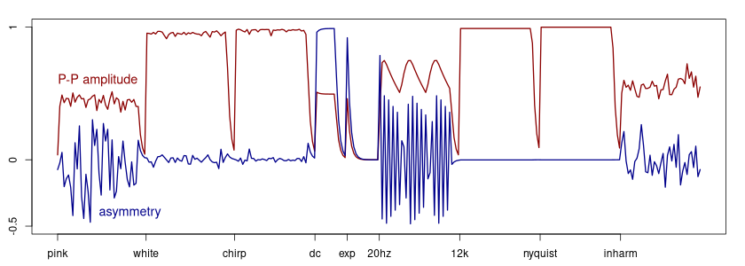
Peak-to-peak amplitude (red) and asymmetry (blue).

As can be seen, the peak-to-peak asymmetry is signed, and is expected to be zero for any sinusoid. If the frequency is too low, the descriptor is unable to average over a whole period and starts tracking the waveform. Here the window length is too short to average out the 20 Hz oscillation.

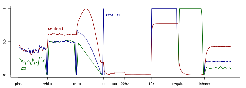
Spectral centroid (red), power difference (blue), and zero crossing rate (green).

It is interesting that some descriptors produce almost exact same values for some signals, but may differ widely for other signals. The power difference, or the centroid of the squared signal, agrees with the normal centroid on pink noise. The centroid turns out to be 0 at the Nyquist rate signal, which is perhaps not expected. The explanation is in the differentiating filter's frequency response. It may also be unexpected that the zcr is 0 at the $f_s/4$ sine, but this happens because a zero crossing is defined as a location where one sample is negative and the one next to it is positive, whereas this signal is $\{1,0,-1,0,\ldots\}$. Since every other sample is zero, no crossing is detected at this frequency.

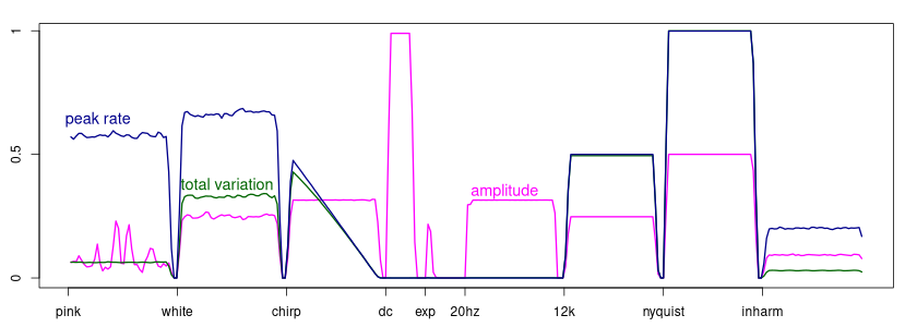
Peak rate (blue), total variation (green), and amplitude as measured with a half-wave rectifier (pink).

The peak rate, or average number of positive peaks, correlates to frequency, at least for sinusoids. The total variation agrees perfectly with the peak rate for sinusoids, including the chirp.

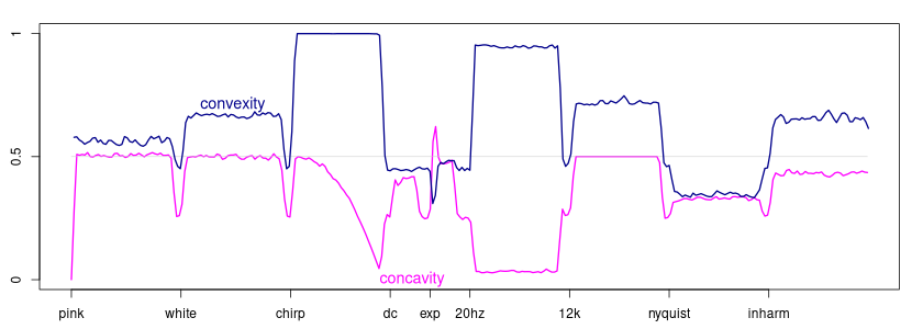
Convexity (blue) and concavity (pink).

Convexity and concavity are complementary and opposite descriptors, but implemented slightly different ways they are not mirror images. As expected, the concavity reaches its highest value for the exponentially decaying signal.

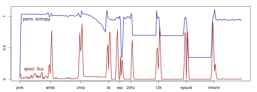
Permutation entropy (blue) and simplified spectral flux (red).

The three-point permutation entropy reaches low values for the exponential decay and the nyqyust rate oscillation. It tends to spike at the boundaries between a signal segment and silence. The spectral flux, using only two frequency bands, responds to all onsets and endings of sounds.

Statistical independence

Many descriptors measure similar things. Depending on the analysed signal, their similarity may be greater or lesser. Instead of using the entire set of signal descriptors, it is often sufficient to use a few that are relatively independent or "orthogonal" to each other.

Two descriptors are independent, with respect to a given class of signals, if their correlation is close to zero. If they are highly correlated one of them may be redundant. Meanwhile, it is important to remember that there may exist another signal which would reveal the difference between the two otherwise apparently similar descriptors.

A practical way to investigate the relative independence is to analyse a sufficiently varied test signal and check all correlations across the set of descriptors. Here we have used the same test signal as above, appended with a few more representative sounds to a total duration of about one minute, analysed using a 4000 point time window (roughly 0.083 sec). The results are as follows.

Strongly correlated descriptors

The following are the descriptors pairs with magnitude of correlation > 0.7:

peak	slope	0.89
cent	powdif	0.88
tv	zcr	0.86
loud	pp-amp	0.84
powdif	mid	0.81
amp	pp-amp	0.79
cent	mid	0.76
convex	cusp	-0.76
slope	zcr	0.75
tv	slope	0.72
loud	amp	0.71
rfsym	nl-asym	-0.70

Abbreviations: cent = spectral centroid, tv = total variation, pow-dif = power difference, cusp = concavity, loud = loudness, nl-asym = nonlinear time series asymmetry, pp = peak-to-peak, rf-sym = rise-to-fall ratio, peak = rate of positive peaks, perm-ent = 3 point permutation entropy, expans = expansion, shim = shimmer, slope = slope sign change.

Weak correlations

These are the pairs of descriptors with magnitude of correlation up to 0.016.

zcr	flux	0.0016
peak	expans	-0.0064
cent	flux	0.0027
expans	mid	-0.0029
rfsym	cusp	0.0053
pp-amp	pp-asym	-0.0071
convex	shim	-0.0074
flux	perm-ent	-0.0076
cusp	pp-asym	-0.01
flux	convex	-0.0102
perm-ent	nl-asym	-0.0105
flux	pow-dif	0.0107
pow-dif	pp-asym	-0.0137
flux	pp-amp	0.0143
perm-ent	mid	0.0158
nl-asym	pp-asym	-0.0162

A few descriptors stand out as having low correlation to most other descriptors. Thus we have pp-asym with its highest correlation to expansion (-0.35); shimmer, most correlated to pp-amp (0.43); and flux, negatively correlated to expansion (-0.44).

The full correlation data set can be found here.

Those descriptors that are weakly correlated to most other descriptors contribute something original to the signal analysis; they are, so to speak, able to recognise traits that other descriptors neglect. One possible way to quantify this effect is to sum the absolute value of the correlations to all other descriptors. The descriptor with smallest sum wins the contest; it is the most independent of the set, as always with respect to the test signal used.

This procedure yields the following descriptors with lowest sum of correlations:

pp-asym	1.089161
flux	1.160496
expans	2.594472
perm-ent	3.324538
shimmer	3.773379
cusp	3.828069

At the other end, slope sign change sums to 7.06, mid to 6.71, and pp-amp to 6.66.

Further ideas

All signal descriptors discussed above produce one output value for each input sample. Averaging over a time window, as they all do, smooths out rapid changes. Therefore, the output can be downsampled in applications such as signal visualisation. Keeping two samples per window length may be sufficient. Downsampling the input signal before sending it to the signal descriptors is worth trying, not only because the time resolution of an audio signal is unnecessarily high for some analysis purposes, but also because many of the descriptors are based on as little as two or three adjacent samples. That makes them sensitive to fast changes in the signal, but in order to capture changes at moderate rates, the input needs to be downsampled.

Some descriptors tend to cluster around some narrow range; when this happens taking the logarithm often reveals their distribution.

Multi-scale analysis is sometimes of interest. Try using the same descriptor with a set of different window lengths to see if scale matters.

These are very low level signal descriptors, but combining a few complementary ones and performing some further statistics on them such as estimating entropy, variance or standard deviation may be all that is needed to make them quite powerful. Some potential use cases are automatic segmentation based on differences between temporal regions, concatenative synthesis, adaptive effects, and adaptive synthesis.

Nonlinear time-series analysis methods are usually more complicated than the ones introduced above. Delay coordinate embeddings are typically used, which are not suitable for inline or realtime processing. The assumption of the nonlinear techniques is that the signal emanates from some dynamical system with reasonably unchanging parameters; otherwise, such methods are inappropriate. However, if an audio signal has been analysed with a set of time domain descriptors, it might be interesting to further analyse these with the help of permutation entropy, visibility graphs, or other techniqes. The standard Fourier transform or autocorrelation should not be forgotten; these could be used to identify periodicities in the descriptor time series.

Source code

The descriptors are implemented as classes with member functions that process input signals one sample at a time and return one output value. As discussed above, these may be optimised for non-feedback usage by making buffered versions where the function is called with an array of samples.

Another potential optimisation would be to lump several descriptors together in a single function call. This may save some workload if more than one descriptor is needed at once, but this is not provided because of the combinatorial explosion of possible combinations of descriptors. If you happen to need some particular combination, it should be easy to restructure them into a single function call.

Download (27 kB zip file)

Acknowledgements

Project realised with support from NKF (såkornmiddel).

References

Literature

Alías, F., Socoró, J. C., and Sevillano, X. (2016). A Review of Physical and Perceptual Feature Extraction Techniques for Speech, Music and Environmental Sounds. Applied Sciences, 2016, 6, 143.
Bandt, C. and Pompe, B. (2002). Permutation entropy: A natural complexity measure for time series. Physical Review Letters, 88(17):174102.
Holopainen, R. (2012). The Constant-Q IIR Filterbank Approach to Spectral Flux. Proc. of the SMC, Copenhagen.
Kantz, H. and Schreiber, T. (2003). Nonlinear Time Series Analysis. Second edition. Cambridge University Press.
Moussallam, M., Liutkus, A., and Daudet, L. (2015). Listening to features. Technical report, Institut Langevin, Paris.
Peeters, G., Giordano, B., Susini, P., Misdariis, N., and McAdams, S. (2011). The timbre toolbox: Extracting audio descriptors from musical signals. Journal of the Acoustic Society of America, vol. 130, no. 5, pp. 2902–2916, November 2011.
Sharma, G., Umapathy, K., and Krishnan, S. (2020). Trends in audio signal feature extraction methods. Applied Acoustics 158 (2020) 107020.