Nonlinear Oscillators and Frequency Modulation
After a brief and elementary introduction to the harmonic oscillator we give some examples of nonlinear and chaotic oscillators and discuss their use in sound synthesis. Then some new examples of FM oscillators are introduced. (See also the page about variants of FM.)
Introduction
Oscillators for musical purposes usually allow for precise control of pitch, although analog oscillators may drift and require a warm up period. Various waveforms such as triangle, sawtooth or pulse can be generated with a constant waveform across the pitch range.
Nonlinear oscillators, known from dynamic systems theory, are quite different. These systems have parameters that determine the system's dynamics, from fixed points to periodic or quasi-periodic oscillations to chaos and global instability. The region of parameter space where there are bounded oscillations is potentially interesting for sound synthesis. In contrast to a normal analog oscillator, in these nonlinear oscillators frequency, waveform and amplitude may all depend on a single control parameter.
To some extent the pitch may be controlled even in nonlinear oscillators. One way to do so is to insert an adaptive mechanism that analyses the pitch at the output and retunes some parameter that affects the pitch so that the oscillator generates the required pitch.
Harmonic oscillators
Differential equations specify the rate of change as a function of the current position $x$ in the phase space (also called state space) of the system. The rate of change is the time derivative $dx/dt$, which we will write as $\dot x$, and the phase space is the set of variables that are involved in the equation, such as the spatial position of a point and its velocity at any given time. Usually a dynamic system has one or more parameters that can take various values in another space, the parameter space. Different kinds of orbits $x(t)$ are traced out depending on the initial condition $x(0)$ and parameters, which are usually supposed to be fixed over time.
The harmonic oscillator is just a sinusoid that oscillates at some amplitude $A$ and radian frequency $\omega$. Recall that the first derivative of $x(t) = \sin \omega t$ is $\dot{x} = \omega \cos \omega t$, and its second derivative is $\ddot{x} = - \omega^2 \sin \omega t$. Combining these facts, we get the second order differential equation $$ \ddot{x} = - \omega^2 x, $$ called a second order system because it involves the second derivative or acceleration. By introducing a new variable $y = \dot x$ we can turn this second order system into the two-dimensional first order system $$ \begin{align} \dot{x} &= y \\ \dot{y} &= -\omega^2x. \end{align} $$ Apart from the initial condition $x(0) = y(0) = 0$ which is a fixed point, any other initial condition will set the system into a permanent oscillation whose amplitude depends on the initial condition.
The harmonic oscillator is an example of a conservative system. One thing that sets conservative systems apart is that the dynamics depend on the initial condition. There is no transient period while the system approaches its final orbit, it starts right on the orbit. This is different from the other type of systems which are called dissipative, where there is an attractor that is gradually approached from a set of initial conditions that belong to the so-called basin of attraction. (If the orbit starts from a point on the attractor itself there is of course no initial transient.) In fact, if a damping term, proportional to the first derivative, is added the the harmonic oscillator, it becomes a dissipative system.
For numerical solution of differential equations we have to take small time steps, of size h, and advance the current value in proportion to the current slope, $$ x_{n+1} = x_n + h f'(x_n), $$ which is the simplest possible numerical scheme, the forward Euler method. This is actually what happens in a digital oscillator when the phase $\theta_n$ is incremented by an amount $\omega$ which is proportional to the frequency: $$ \theta_{n+1} = \theta_n + \omega. $$ The frequency of course is the derivative of the phase.
Ordinary differential equations cannot produce instantaneous jumps from one value to another. In sound synthesis, this smoothness implies that the spectrum will not have too strong high frequency components, so aliasing is usually not a great concern. However, it is possible to have rather snappy changes in ordinary differential equations too. Such fast changes happen when the derivative briefly becomes very large. When large derivatives occur, the simple Euler method may become unstable and one has to resort to better numerical schemes.
Nonlinear oscillators
van der Pol
The van der Pol oscillator is similar to an harmonic oscillator, except for a nonlinear damping term. It is often written as the second order system $$ \ddot{x} = - \mu (x^2 - 1)\dot{x} - x $$ with parameter $\mu \geq 0$. This oscillator illustrates the way amplitude, wave shape and frequency all depend on the parameter. As the parameter increases, the pitch drops while the amplitude of $x$ increases and the waveform transforms from a sinusoid to a spikey pulse train.
Sound example. Van der Pol oscillator with parameter sweep $0 < \mu < 4$.
It will be useful to convert the system into first order form, which is $$ \begin{align} \dot{x} &= - \mu (y^2 - 1)x - y \\ \dot{y} &= x. \end{align} $$ One possible variation is to smooth out the nonlinear damping term by the introduction of a new variable, $\dot {z} = y^2 - 1 - z$. This by itself does not make much of a difference, but adding an input to the system does. With a sinusoidal forcing with amplitude a and frequency $\omega$ applied to $y$ we have: $$ \begin{align} \dot{x} &= -\mu zx - y \\ \dot{y} &= x + a \sin(\omega t) \\ \dot{z} &= y^2 - 1 - z. \end{align} $$
Sound example. Van der Pol oscillator with parameter sweep $1 < \mu < 3$ and driving by a sinusoid that begins at 400 Hz, then rises during the second half.
With the presence of the forcing term this system may become chaotic, which can be heard in many parts of the last sound example. It should be noted that the inclusion of the driving term makes this a four-dimensional system, which might potentially be hyper-chaotic at some parameter values.
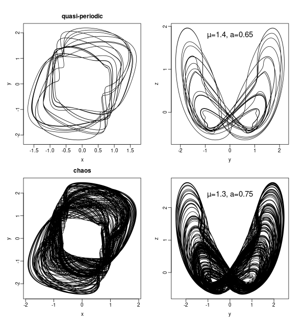
The forced van der Pol oscillator with driving frequency 500 Hz. Top: at $\mu = 1.4$ and $a = 0.65$ the orbit is quasi-periodic. Bottom: $\mu = 1.3$ and $a = 0.75$ produces chaos. Left plots show the (x,y) plane, right plots the (y,z) plane.
Nosé Hoover
Let us take a look at a conservative system, the Nosé-Hoover oscillator: $$ \begin{align} \dot{x} &= y \\ \dot{y} &= yz - x \\ \dot{z} &= 1 - y^2 \end{align} $$ An initial condition producing a chaotic orbit is (0, 0.1, 0).
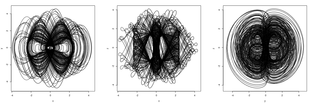
The orbit of the Nosé-Hoover oscillator as seen, left to right, from the $(x,y), (x,z)$ and $(y,z)$ planes. If one would trace a the orbit over a longer time it would fill up the space in a compact blob.
Sound example. Nosé-Hoover oscillator in standard form.
Sprott has proposed a generalisation of this system where the last equation is replaced by $\dot{z} = 1 - |y|^b $, which appears to be chaotic for all $b > 1$. The size of the orbits (i.e. the amplitude of each of the variables) shrinks as b increases. The constant term 1 may also be replaced by a parameter $a \approx 1$ in order to have a more flexible system of the form $$ \begin{align} \dot{x} &= y \\ \dot{y} &= yz - x \\ \dot{z} &= a - |y|^b. \end{align} $$
Sound example. A characteristic Nosé-Hoover sound at parameters $a=0.7, b=1.5$.
Sound example. Parameters $a=1.2, b=3$. Notice moments of near-periodicity.
We know that the original Nosé-Hoover oscillator is a conservative system which is chaotic for some set of initial conditions, and (quasi-)periodic for other initial conditions. For the purpose of sound synthesis it will be interesting to vary the parameters over time, but there is a caveat. The classification of orbits as periodic, quasi-periodic or chaotic applies to systems with constant parameters. Changing a parameter slowly over time means that the system will be on its way to a new attractor if it is dissipative, or may transit from chaos to quasi-periodicity or periodicity in the case of a conservative system.
Sound example. The Nosé-Hoover oscillator with $a = 1$ and $b = 1$ exhibits a brief chaotic transient before landing on a periodic orbit.
Chaotic transients eventually landing on periodic orbits is the hallmark of dissipative systems. If such transients were to occur in a system known to be conservative, the conclusion must be that the numerical integration scheme is not good enough.
Toda oscillator
We have seen how an harmonic oscillator can be written as a second order system or as a two-dimensional first order system. Third order systems are called jerk systems, since jerk is the term for the third derivative (then there are higher orders, called snap, crackle and pop).
The Toda oscillator may be formulated as the jerk system $$\dddot{x} = -\ddot{x} - a\dot{x} - \exp(x) + 1.$$ It is more convenient to convert it to the standard three-dimensional form $$ \begin{align} \dot{x} &= y \\ \dot{y} &= b z \\ \dot{z} &= 1 - e^x -ay - z \end{align} $$ with parameters b and a.
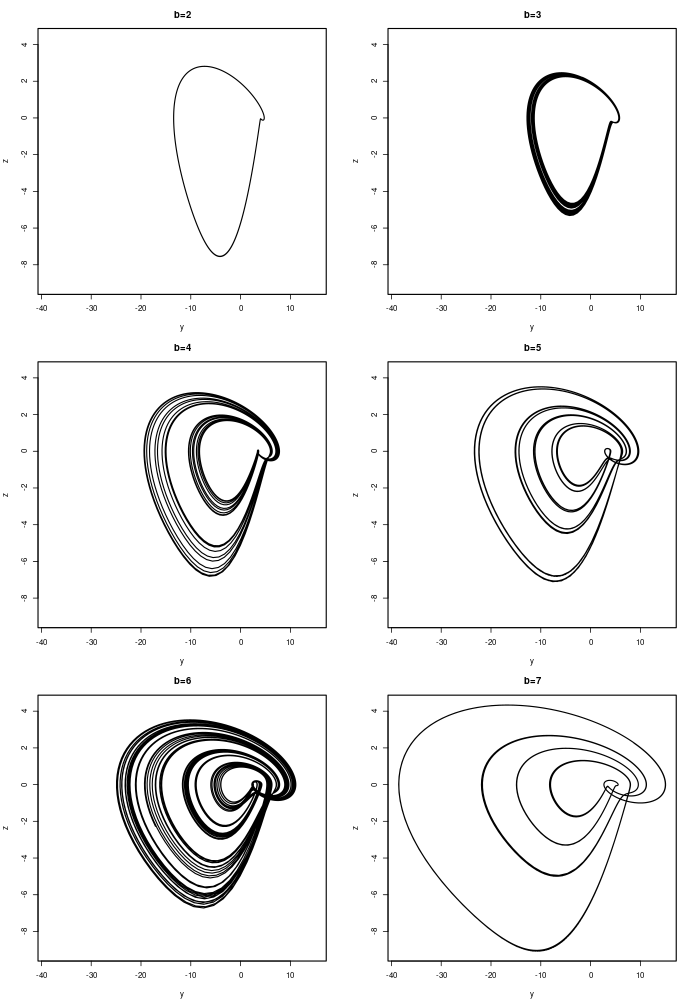
Several attractors of the Toda oscillator with $a=0.25$ and $b=2, \ldots, 7$ displayed in the $(y,z)$ plane.
All orbits are highly asymmetrical, going much farther in the negative than in the positive direction. The x and y coordinates also have larger amplitudes than the z coordinate. Apparently, the amplitude of the z coordinate does not change nearly as much as the other two coordinates as a function of the parameters, which makes it a good choice for sound synthesis.
Sound example: Symmetric parameter sweep of parameter b, increasing linearly from 1 to 8, then reversing and decreasing back to 1 in the left channel. The right channel is just the time-reversed version of the left channel. As a consequence, the parameter b always takes the same value at any given time in both channels. If the orbits were always perfectly symmetric in time the two channels would be identical apart from some constant phase shift. Chaotic parts stand out as a broadening of the stereo image caused by decorrelation.
Like many other systems, the Toda oscillator can take external forcing by a sinusoid (or any other driving signal). The system then takes the form $$ \ddot{x} + d\dot{x} + e^x -1 = F \cos(\omega t) $$ with parameters $d, F, \omega$ representing damping, forcing amplitude and frequency.
Phase coupled oscillators
Examples of synchronisation can be found in many situations, such as pedestrians walking over a bridge, an applause at a concert, or two organ pipes that are just slightly detuned. Kuramoto's model of phase coupled oscillators is widely studied. Although rarely mentioned in the context of sound synthesis, it can be used on its own or, as we will do here, as an additional way of connecting FM oscillators.
When all oscillators are phase coupled to each other with equal strength, the equation of a system of N oscillators is $$ \dot{\theta}_i = \omega_i -\frac{K}{N}\sum_{j=1}^{N} {\sin(\theta_i - \theta_j)}, $$ where K > 0 is the coupling strength. The frequencies $\omega_i$ are usually taken from a unimodal probability distribution centred at 0. Another interesting idea is to use the Kuramoto system as an additive synthesis model with interaction between all oscillators. With the coupling strength set to zero, the output is a sum of pure sinusoids, and with positive coupling their interaction causes intermodulation effects. This was explored in the first half of the piece Jazz Nonstandards from Signals & Systems.
The degree of synchronisation between the oscillators is quantified by the complex order parameter $$ R e^{i\psi} = \frac{1}{N} \sum_{k=1}^{N} e^{i\theta_k} $$ where $\psi$ is the average phase and $R \in [0,1]$ is the radius, with higher radii indicating a more synchronised state.
Hybrid Circle Map with Feedback FM
The Circle map is a simple dynamic system that exhibits several types of bifurcations and other phenomena such as mode locking, or the tendency to lock in to a certain frequency in a region of its parameter space. Although it has been proposed for use in audio synthesis (in a paper by G. Essl), it is recalcitrant in the way most chaotic maps are. The circle map $$ \theta_{n+1} = \theta_n + \Omega - K \sin (\theta_n) $$ has a frequency term $\Omega$ and a nonlinear feedback term with coupling strength K. For $| \Omega | \leq |K|$ there is a slight chance that the system might stop oscillating, since when $\Omega = K \sin \theta_n$ the phase increment becomes zero.
For sound synthesis purposes the term $\sin \theta_n$ can be taken as the output signal. Since the circle map equation describes a more or less perturbed phase update of an oscillator we could actually use it as such. But we will add another twist and combine it with feedback FM: $$ \theta_{n+1} = \theta_n + \Omega - K x_n \\ x_{n+1} = \sin (\theta_n + \beta x_n). $$ Notice that this system reduces to feedback FM if $K=0$, whereas for $\beta=0$ it reduces to the circle map.
Using a trick that was introduced for taming feedback FM, a simple lowpass two-point average filter can be inserted in the feedback loop. The addition of this filter raises the system's dimension from a 2D to a 3D map, and it also has a prominent effect on the dynamics, and generally, the sound. The system thus becomes: $$ \theta_{n+1} = \theta_n + \Omega - Ky_n \\ x_{n+1} = \cos(\theta_n + \beta y_n) \\ y_{n} = 0.5 (x_n + x_{n-1}) $$ This system tends to produce high pitched tones, and white or coloured noise. But the transitions as the parameters are swept through some range are not by far as abrupt as for the simpler 2D version.
The two following examples are rather loud.
Sound example. Feedback FM with circle map, original 2D-system.
Sound example. Feedback FM with circle map, version with two-point average filter.
These two sound examples illustrate the difference between the 2D-system and the filtered version. All parameters change identically over time between the two examples.
Cross-coupled FM
Next we will consider a few systems combining cross-coupled feedback and phase coupling.
First, let us consider the simple system $$ \dot{\theta}_c = \omega_c (1 + J y) \\ \dot{\theta}_m = \omega_m (1 + J x) $$ where either or both of the signals $$ x = \sin (\theta_m + \phi ) $$ $$ y = \sin (\theta_c + Ix) $$ can be taken as the audio output, and $\phi$ is an input from an external modulation source. Any signal can be used for external modulation, in particular, this could be a way to connect several instances of this system. Apart from the carrier and modulator frequencies, the parameters are the feedback index $J$ and modulation index $I$. Notice that $J \geq 1$ may cause oscillation death.
This system can be extended with feedback from each oscillator to itself. In a previously described system we introduced coupling parameters c (cross terms) and b (self-modulation) in the coupled system $$ x_{n+1} = \sin (\theta_n + b_1 x_n + c_1 y_n) \\ y_{n+1} = \sin (\varphi_n + b_2 y_n + c_2 x_n) $$ in which the phases $$ \theta_{n+1} = \theta_n + \omega_1 - K \sin (\theta_n - \varphi_n) \\ \varphi_{n+1} = \varphi_n + \omega_2 - K \sin (\varphi_n - \theta_n) $$ increase with each their own frequency while also being phase coupled with coupling strength K. (This system was probably used in one of the three simultaneous layers in the piece Teem Work originally composed in 2013. Unfortunately the source code for the piece has been lost.)
Bifurcation plot for cross-FM. Colour legend: Period 1, gray; period 2, orange; period 4, blue; period 3, bright yellow, chaos, red. On the horizontal axis, $-1 < c_1 = c_2 < 4$, vertical axis: $-0.5 < b_1 < 5$ and $b_2 = 0.5$ (constant). The modulator and carrier frequencies are both 0; hence the coupling term does not influence the dynamics.
Dual coupled system
This system has four phase variables $$ \dot{\varphi}_i = \Omega_i + J \sin \theta_i - K \sin (\varphi_i - \theta_i) \\ \dot{\theta}_i = \omega_i + M \sin \theta_{i+1} - K \sin (\theta_i - \varphi_i) $$ with $i=1,2$ and the seven parameters $\Omega_i, \omega_i, J, K, M$. For more control the indices J, K, M may be separated for each i as if the original parameter space is not complicated enough. Again it may be useful to look for parameter combinations that may result in silence, which amounts to finding parameter values for which the right hand side of all four equations simultaneously evaluate to zero. Suffice to say that oscillation death remains a possibility. It should not be hard to find a plethora of bifurcation types by varying one or more of the parameters.
This system can be regarded as having two subsystems that are connected with variable strength through the $M$ and $K$ parameters. For $M = K = 0$ this reduces to a dual two-oscillator FM system.
Triple system
Here the complete system consists of six phase variables and the equations $$ \dot{\varphi}_i = \Omega_i + J \sin \theta_i - K \sin (\varphi_i - \theta_i) \\ \dot{\theta}_i = \omega_i + M \sin \theta_{i+1} - K \sin (\theta_i - \varphi_i) $$ for $i=1,2,3$. The parameters are the three pairs of frequencies $\Omega_i, \omega_i$, the modulation index J, and the cross-coupling indices K and M. As with the dual system above, the same remarks apply about possible oscillation death and the plenitude of bifurcation scenarios that might be encountered in this system.
As the number of phase variables and oscillators grow, the number of ways these may be interconnected increases even more. A few types of graphs or networks of oscillators have been studied in the quite extensive literature on synchronisation and may provide ideas for further experimentation.
The three systems above, the cross-coupled, the dual and the triple system, can be heard in action in a piece called The Final Countdown.
Quasiperiodic linear ODE
The idea of using a linear ODE with quasiperiodically modulated coefficients as the basis for sound synthesis was explored in a piece called The Quasi-periodic Table. Despite being a linear system, intermodulation between frequencies which otherwise is typical in nonlinear systems can be found here as well.
Let $Z\in\mathbb{C}^{n}$ be the state variable and $Q_{t}\in\mathbb{C}^{n\times n}$ be a matrix with coefficients of the form $$ q_{ij}(t)=\sum_{k}a_{k}\exp(i\omega_{k}t) $$ whose frequencies $\omega_{k}$ are incommensurate both within a single matrix coefficient and across different coefficients. The system is then given by $$ \dot{Z}=Q_{t}Z. $$ It may not be evident why this system produces intermodulation between the frequencies present in the matrix coefficients, or that its stability depends in some way on the initial condition. (For an in depth discussion of this kind of systems, see Haken's Synergetics book.)
In The Quasi-periodic Table $Z\in\mathbb{C}^{2}$ and two of the matrix elements consist of one single complex exponential each, the other two use a sum of two complex exponentials. Still, with as little as six quasi-periodic frequencies present in the matrix Q, surprisingly rich spectra can be obtained.
Conclusions, if any
Nonlinear oscillators are interesting sound sources where amplitude, frequency and waveform typically are not independently controllable. External inputs can be used, sometimes with the result that the oscillator synchronises to the input. There are already some chaotic oscillators available for modular synthesizers. For experimentation with various systems one can easily solve the equations numerically.
Literature
- Essl, G. (2006). Circle Maps as a Simple Oscillators for Complex Behavior: II. Experiments. Proc. DAFx-06, Montreal.
- Haken, H. (2004). Synergetics. Introduction and advanced topics. Springer.
- Ott, E. (2002). Chaos in Dynamical Systems. Second Edition. Cambridge University Press.
- Slater, D. (1998). Chaotic Sound Synthesis. In: Computer Music Journal 22.2, pp. 12–19.
- Sprott, J.C. (2010). Elegant Chaos. Algebraically Simple Chaotic Flows. World Scientific.
- Stefanakis, N., Abel, M., and Bergner, A. (2015). Sound Synthesis Based on Ordinary Differential Equations. Computer Music Journal 39:3, pp. 46–58.
- Strogatz, S. (1994). Nonlinear Dynamics and Chaos. Westview.
© Risto Holopainen 2020