A small but complex world of self-organising oscillators
The Bourgillator is a system of interacting oscillators expressed as an autonomous ordinary differential equation. It came about in an attempt to construct a simple, medium sized system which should be inherently unstable and wander between a number of qualitatively different states. Each oscillator is associated with three variables: Apart from its phase $\theta$ it has an instantaneous amplitude a and a slow variable A which measures the amplitude at the output of the oscillator over the recent past. A discontinuous function of the slowly changing amplitude envelope influences both the frequencies and the amplitudes of each oscillator. The discontinuity works like a switch that allows the oscillators to jump between different pitches.
In a sufficiently general form, the Bourgillator is described by the equations $$ \dot{\theta}_i = f_i (\boldsymbol{A}) - K_i(\boldsymbol{A})\sum_j {w_{ij}\sin(\theta_i - \theta_j)}$$ $$ \dot{a}_i = g_i(\boldsymbol{A}) - a_i^p$$ $$ \dot{A}_i = \frac{1}{\tau}(x^2_i - A_i)$$ where $i = 1, 2, \ldots, N$. The oscillators are arranged on a circle such that $\theta_{N+1} \equiv \theta_1$ etc. $\boldsymbol{A}$ denotes the full vector $(A_1, A_2, \ldots, A_N)$, and $a_i^p$ is a damping term with p a small positive integer.
A modified version of the Kuramoto system should be easily recognisable in the first equation. Here, however, the oscillators' internal frequencies are drifting rather than fixed, and so is the amount of coupling. When the phase coupling is large enough the oscillators will tend to synchronise.
The oscillators' output $$ x_i(t) = a_i(t) \sum_k {\alpha_k \cos(\Omega_k \theta_i(t) + \phi_k)} $$ is an amplitude modulated periodic or quasi-periodic function, a sum of sinusoids with frequencies $\Omega_k$ which may or may not be harmonically related. The average output amplitude is captured by the slow variable $A$, which should be thought of as an envelope follower. The constant $\tau \gg 1$ sets the time scale of the envelope follower; the bigger it is, the slower the envelope follower reacts to the incoming signal.
Both g and f are discontinuous functions; in particular $$ g_i(A) = \sum_j {\beta_j \Theta(A_i - A_{i+j})}$$ where $\Theta(x)$ is the Heaviside step function, equal to 1 if $x>0$ and 0 if $x\leq0$. The function f in fact uses a modified form of g.
The source code (which may not be very useful for purposes other than documentation) is now available along with a few sound examples generated by different versions of the program.
The composition
A composition also titled Bourgillator was realised using a variant of the above system in May 2017. In this case 21 oscillators were used. There is a surround mix where the oscillators are distributed to five channels, as well as a sixteen channel version and a stereo version.
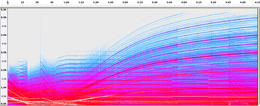
As seen in the sonogram there are a few abrupt transitions, most of which happen near the beginning, but a few occur several minutes into the piece. After about one minute some oscillators enter a long process of gradually rising frequencies while another sub-population of oscillators remain more or less at a fixed frequency. At some earlier point the system also splits into a group of very quiet oscillators and a group of loud oscillators. This spatial differentiation into two distinct populations of oscillators can be described as a process of self-organisation.
For this particular realisation, the oscillator's output is a scaled sum of the first three harmonic partials. The frequency is given by the somewhat complicated function $$ \dot{\theta}_i = \omega_i + \sigma \Delta_i(A)g_i(A) - K(A) \sum_j w_{ij}\sin(\theta_i - \theta_j)$$ for which we have introduced some auxilliary variables and constants. In the absence of other perturbations, each oscillator would run at its own frequency $\omega_i$ which is chosen randomly in the range -50 to +100 Hz. The drift term $$ \Delta_i(A) = 1 + \frac{1}{2}(A_{i-1} - A_{i} + A_{i+1}) $$ multiplies the step function g. Each oscillator's phase is connected to its two nearest neighbours with $w_{ij} = 1$, and to the oscillator on the opposite side of the circle by alternating positive and negative coupling depending on whether i is odd or even, i.e., $w_{ij} = (-1)^i$ if $j = i + N/2$. The phase coupling $$ K(A) = c \sqrt{A_i + A_{i+N/2}}$$ varies in strength in proportion to the sum of the current and opposite oscillators' amplitude envelopes.The amplitude equation takes the straightforward form $$ \dot{a}_i = g_i(A) - \gamma a_i^2 $$ where $\gamma$ is a small positive constant. The envelope follower A is as specified above. Finally, the step function $$ g_i(A) = \sum_{j=1}^{N/3}2^{-j}\Theta(A_i - A_{i+j}) $$ only sums over a third of the oscillators with decreasing weights. Notice that $g_i$ is maximised when oscillator i is the loudest one among the subset of oscillators which are compared under the sum, and is minimised when the oscillator is the quietest one. Whenever the amplitude of an oscillator $A_i$ increases past the amplitude $A_j$ of another oscillator which was previously louder, the relative order of the amplitudes changes, which causes a jump in the value of $g_i$ by various amounts depending on the oscillator's relative position along the circle.
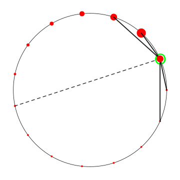
The figure on the left illustrates the connectivity. The current node (encircled by green) is connected to its two nearest neighbours on either side with a reinforcing coupling, and to the node on the opposite side with alternating positive and negative coupling. Negative or contrarian coupling causes the oscillators to avoid synchronisation. The diminishing sizes of the nodes indicates the relative magnitude of the $\beta_j$ coefficients as seen from the current node. When the current oscillator's amplitude overtakes that of its closest left neighbour, $g_i$ will increase by the greatest amount possible.
The other parameters that have to be specified are the strength of frequency fluctuations $\sigma$, the damping term $\gamma$ which keeps the amplitude growth in check, and the coupling strength c. Along with the randomly chosen distribution of oscillator frequencies, this parameter space allows for a number of different temporal developments of the system. Finding an interesting enough piece of sonic evolution in this parameter space is not necessarily easy. The composition was found after some trial and error, not just by trying different parameter values, but by exploring a number of different forms of coupling and frequency drift functions. Substituting other forms of the equations the Bourgillator may become a Bougrillator, and that is quite a different beast.
A 16 channel version of Bourgillator was premiered at Zeppelin, arranged by Sonoscop on November 3, 2017 where this as well as many other pieces are available for listening.
© Risto Holopainen 2017