New waveforms for the people!

Wavetable oscillators can hold virtually any waveform—preferably bandlimited waveforms if aliasing is a concern. Although some of the waveforms introduced here are not bandlimited, most of them have a steep spectral slope and can be used at low fundamental frequencies (in particular, as LFO waveforms) without disturbing amounts of aliasing. Some of the waveforms might be suitable for direct generation by the equations given here if one wants to modulate their parameters without having to interpolate between lots of wavetables.

For an introduction to the concepts of wavetable synthesis, the recommended reading section is a good place to start.

The waveform library

All the waveforms introduced below and many more have been implemented in C++ together with a simple linearly interpolating wavetable oscillator. If you want to play with the code, download it and include it directly in your projects. No complicated compilation process is required. The code is licenced under GNU GPL v.3. Modifications and improvements are encouraged. Absence of errors or bugs is not guaranteed, nor is general usefulness.

Good wavetable manners

The wavetables are written to an array expected to be of type double, float, or long double, and of odd length (such as a power of two plus one). The first and the last entry of the array will be identical, because the wavetables are designed to be used with linearly interpolating oscillators that need the extra guard point at the end.

Wavetables have been used for sound synthesis for a long time because of the enormous efficiency gain compared to direct additive synthesis. Instead of summing a large number of sinusoids, the waveform is pre-calculated and put in a table which is accessed by the phase variable of an oscillator. Wavetables are best suited for perfectly harmonic sounds, but inharmonic sounds may be created by using two or more detuned oscillators that access different partials as in group additive synthesis.

Another way to detune one or a few partials slightly involves the use of several wavetables. Each table contains the same partials in the same phases, except for the set of detuned partials which each lag or lead in phase by the same amount between adjacent wavetables. Reading the wavetables cyclically makes the partials with phase offsets detuned with respect to the other partials.

Timbral morphing is possible by interpolating between two or more wavetables that store timbral variants. Similarly, for an oscillator to sound homogenous across a wide frequency range, a set of wavetables should be defined. For low fundamental frequencies the wavetable should contain many partials, and as the fundamental frequency rises the number of partials should decrease correspondingly.

Since the wavetable will be read at different speeds it makes no sense to define its sampling rate as such, but the sampling theorem still means that the highest partial that can put in the table will need at least two samples to complete one period.

Let $w_n = \sin (k2\pi n/L)$ be a sinusoid stored in the wavetable where $n = 0, 1, \ldots, N-1$ is the sample index, L is the wavetable's length and k is the partial number. Then the highest partial would be at $k = L/2$, but this would not be very useful since the samples $ \sin(\pi n) = 0 $ would be put into the table. Therefore it is better to limit the highest partial to a fourth of the table size or, preferably, even lower.

Waveforms may be generated in the time domain or by adding sinusoids in the frequency domain. When harmonically rich sounds free from aliasing are sought, one must use bandlimited waveforms. Choose a waveshape, find its Fourier series, and add up a limited number of partials to make a stricty bandlimited waveform. In the time domain the spectral slope can be controlled by putting constraints on the smoothness of the wave shape. This is done by assuring that derivatives of increasing order are continuous; the higher the order of continuous derivatives, the steeper the spectral slope.

In particular, a periodic function with a finite number of discontinuities has a Fourier series with terms proportional to $1/k$ where k is the partial number; a function with piecewise continuous derivative has terms of the order $1/k^2;$ and in general a function whose N-1 first derivatives are continuous but whose Nth derivative is not continuous has a spectrum that drops off like $1/k^{N+1}.$

Even bandlimited functions will alias if the wavetable oscillator is run at a frequency that makes the highest partial exceed the Nyquist frequency with results ranging from dreadful to inaudible. Fortunately wavetable synthesis, unlike nonlinear synthesis techniques, can always be made bandlimited.

When using non-bandlimited waveforms such as some of those described below, one could generate a fairly long wavetable, take its FFT and truncate the spectrum, then do an inverse FFT to get a bandlimited waveform. This waveform can be further downsampled and put into a wavetable simply by picking every 1 of N samples in such a way that the waveform is oversampled. Although a recommended procedure, this is not implemented in the wavetable library.

There is also quantisation noise to worry about. Use a longer wavetable and interpolation for cleaner sounds.

Waveform catalog

Most of the common classical bandlimited analog waveforms (square, triangle, saw, pulse) have been implemented in the library but will not be discussed here.

Notice that the functions are defined over different ranges. Sometimes they are defined over the integers 0 to $N-1,$ where N is the table size, but often it is more practical to define them over the continuous interval $[0,1]$ or $[-1,1].$ The function then is sampled at N points and written to the table.

All functions are templates with the definition template <typename REAL> where REAL is expected to be a floating point type.

Expogliss

void make_expogliss(REAL *wt, int N, uint p=5, REAL r=8.0, bool norm=true)

The idea is to generate a smooth waveform which oscillates at a rising frequency while decaying in amplitude. This waveform is continuously differentiable but not bandlimited and takes two parameters, $p \in \mathbb{N}$ and $r > 1.$ A diffuse formant may appear around p times the fundamental when r is set to relatively low values.

Note sequence using the expogliss waveform.

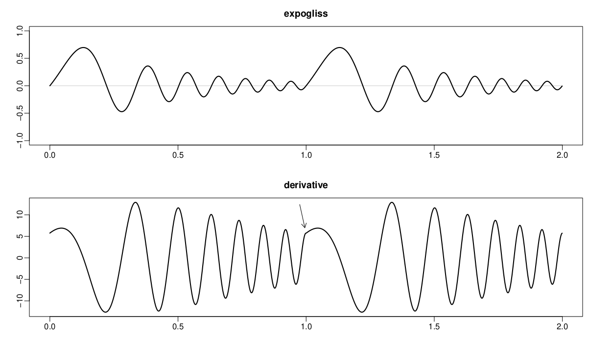
Top: two periods of the waveform. Bottom: The derivative of the waveform. The arrow points where the derivative has a corner which makes the second derivative discontinuous.

The wavetable will contain p periods in total of an exponentially decaying sinusoid with rising frequency, covering the frequency range r. The frequency will start off at its lowest, $2\pi\omega_{0},$ and reach $2\pi(\omega_{0}+2)$ at the end of a full period. Working backwards, we have the frequency range $r=\omega_{1}/\omega_{0}$ or $$\omega_{0}=\frac{2}{r-1},$$ where we assume that $r>1.$

Define the waveform as a function $f(t),\ t\in[0,1].$ First the exact right number of periods, p, will be fit into the interval $t\in[0,1]$ so that the slope of the waveform will have the same sign at the beginning and the end. Finally, multiply the waveform with an envelope that ensures that the slopes at the beginning and the end are identical.

First we generate the sinusoid $$x(t)=\sin\gamma\theta_{t} \qquad (1)$$ with variable frequency $\omega_{t}=\gamma\dot{\theta}_{t},$ where $\gamma$ is a constant to be determined. Setting $\omega_{t}=\omega_{0}+2t,$ the phase at time t is found by integrating $\dot{\theta}=\omega_{0}+2t$ from the initial condition $\theta_{0}=0,$ giving $$\theta_{t}=\intop_{0}^{t}\omega_{0}+2\tau \,\mathrm{d}\tau=\omega_{0}t+t^{2}. \quad (2)$$ As t goes from $t=0$ to $t=1$ the sinusoid $x(t)$ should complete p entire periods (of decreasing length). Therefore the phase $\gamma\theta_{t}$ in (1) must reach $2\pi p$ when $t=1.$ From the integral (2) we see that $\theta_{t}|_{t=1}=\omega_{0}+1,$ whence $$\gamma=\frac{2\pi p}{\omega_{0}+1}.$$

In order to have a continuous derivative where the table wraps around at the end points $f(0)=f(1)$ we evaluate the derivative $$x'(t)=\gamma(\omega_{0}+2t)\cos(\gamma(\omega_{0}t+t^{2}))$$ at the end points $x'(0)$ and $x'(1).$ Since the increasing frequency makes $x'(1)$ greater than $x'(0)$ we multiply $x(t)$ with a decaying amplitude envelope $e^{-\lambda t}$ with decay parameter $\lambda > 0$ chosen such that the slopes at the end points match, that is, $f'(0)=f'(1).$ Solving $x'(0)=e^{-\lambda}x'(1)$ for $\lambda$, we find that $$\lambda=\ln\left(\frac{x'(1)}{x'(0)}\right)$$ and the waveform becomes $$f(t)=e^{-\lambda t}\sin(\gamma(\omega_{0}t+t^{2})),\ t\in[0,1].$$ This waveshape is once continuously differentiable but its second derivative is discontinuous where the wavetable wraps around.

Here the oscillator makes a slow glissando using the expogliss waveform with parameters $p=12, r=3.5.$ At the end the frequency becomes negative and the waveform actually can be heard to reverse direction and go backwards.

Smooth bump functions

void make_bump(REAL *w, int N)
void make_symbump(REAL *w, int N)
void make_diffbump(REAL *w, int N, bool norm=true)

Bump functions are smooth and have compact support (they are zero outside of some finite interval). The first one generates the positive function $$w_{t} = \exp\left(1-\frac{1}{1-t^{2}}\right),\quad t\in[-1,1]$$ which has continuous derivatives of all orders.

The second one makes a function with the same symmetry as a sinusoid by following the bump function as defined above with a negative copy of itself.

When differentiated, the positive bump function remains smooth but turns into a bipolar function. Its shape is similar to that of a sawtooth, but less sharp.

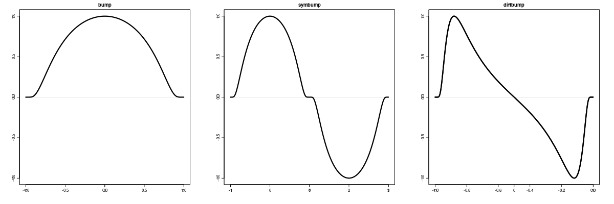
From left to right: the positive bump function, a symmetric bipolar variant and the derivative of the bump function.

Note sequence starting with the symmetric bump waveform and gradually morphing into the differentiated bump.

Formant

void make_formant(REAL *wt, int N, int c, bool norm=true)

With some abuse of terminology, put a "formant" frequency at partial c. (Real formants do not generally move along with the fundamental frequency.) Creates an almost symmetrical spectrum centered around the partial c; surrounding partials decay roughy as $a_{k} \sim 1/|k-c|^{2}.$ A few extra partials are added to the high end of the spectrum. $$w_{n}=\sum_{k=1}^{p}a_{k}\sin(k2\pi n/N)$$ $$a_{k}=\frac{1}{|k+1/2-c|\times|k-1/2-c|}.$$

Formant waveform centered at the sixth partial. The vibrato is generated with an LFO running the twin peaks waveform described below.

Twin peaks

void make_twinpeaks(REAL *wt, int N, bool naive=false, bool norm=true)

Named after its strong first and second partials.

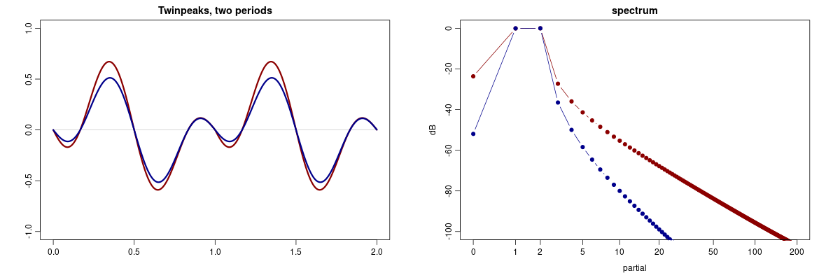
Waveforms and spectra of naïve version (red) and improved version (blue).

Take the difference of two sinusoids whose periods do not fit into the wavetable and multiply with a function that makes the waveform continuous (naïve version) or that also makes the waveform's slope continuous (improved version).

Define the function $g(t), 0 \leq t \leq 1,$ as the difference $$ g(t) = \sin (5\pi t/2) - \sin (7\pi t/2) $$ and, for the naive version, multiply it with the ramp function $r(t) = (1-t).$ This will make the endpoints of the waveform meet, but there will be a corner where the slope changes suddenly.

For the improved version, multiply $g(t)$ by a function $p(t)$ such that the derivative $\frac{d}{dt} (p(t) g(t))$ coincides at the end points $t=0$ and $t=1.$ Furthermore, we require that $p(1) = 0$ and $p'(1)=-1.$ Taken together, these constraints can be met with a quadratic polynomial $p(t).$ Solving for the coefficients using the constraints, we have $$p(t) = (c-1)t^2 + (1-2c)t + c$$ where $c=2/\pi$ and $$w_{t} = p(t) g(t), \qquad t\in[0,1]$$ is the final waveform.

In contrast to the naive version where the third partial is about 27 dB below the first two partials, in the improved version it is about 36 dB below. Both versions have a small DC offset, but it is much smaller for the improved version.

Chirp

void make_chirp(REAL *wt, int N, REAL c=5, REAL B=12.5)

Twin peaks waveform with vibrato generated by the chirp function.

Generates a chirp or fast downwards glissando multiplied by a window function. In the middle of the waveform when the window funcion reaches its maximum, the instantaneous frequency (in partial numbers) is c. The frequency sweeps linearly from $2c$ down to zero.

The waveform $$ w_t = A(t) \sin (2\pi \varphi_t), \quad t \in [-1,1] $$ is constructed by integrating the phase $$ \dot{\varphi} = 2c (1 - \frac{t+1}{2}) $$ and multiplying by the window function $$ A(t) = \frac{1}{1 + \beta t^2} - \frac{1}{1 + \beta}. $$ The parameter $\beta \geq 1$ sets the steepness of the window function; at higher values the window focuses on a narrower region.

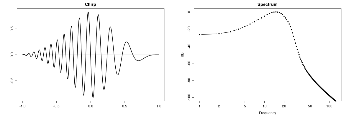
Chirp function and its spectrum, here with $\beta=5$ and $c=7$.

Diphone

void make_diphone(REAL *wt, int N, uint P=5)

Splice two sinusoid segments of equal length together. The first half consists of one period, the second half contains P periods. Match the slopes at the joint by multiplying the amplitude of the second segment by $1/P.$ Hence, $$ w_t = \begin {cases} \sin(2\pi t), \quad & t \in [-1,0) \\ \frac{1}{P} \sin(P2\pi t), \quad & t \in [0,1]. \end {cases}$$ Apart from a strong second and $2P$th partial, the spectrum consists of odd partials. diphone

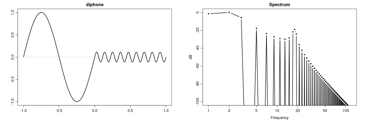
Diphone waveform and spectrum with $P = 9.$

Slow transition between two diphone waveforms, the first with 12 cycles in the second half of the waveform, the second one with five cycles.

Half-sine

void make_halfsine(REAL *wt, int N, int P=25, bool norm=true)

This waveshape is derived from the Fourier series of one period of a sine wave followed by an equal length of silence. Similarly to the diphone family of waveshapes it has a strong second partial and odd partials with amplitudes roughly proportional to $1/k^2.$

Note sequence using the half-sine waveform.

Quadratic map

void make_noise(REAL *wt, int N, double seed=1/7.)

Generates a noisy signal by iterating the chaotic quadratic map $$w_{n+1}=2w_{n}^{2}-1$$ from the initial condition (seed) $w_{0} \in (-1,1);$ the default initial condition is $w_{0}=1/7.$ By a change of variables this map can be transformed into the logistic map.

With a sufficiently long wavetable and at low oscillator frequencies no periodicity will be audible. Aliasing will be noticed at higher frequencies. This is not the kind of signal one would normally think of putting into a wavetable for oscillators.

The Volterra function

void make_volterra(REAL *w, int N, bool norm=true)

A quirky function often mentioned in real analysis (perhaps in a slightly different form) is $$w_{t}=t^{2}\sin(\pi/t),\quad w_{0}=0$$ which we define over $t \in [-1,1].$ Dividing by t causes the frequency to approach infinity near zero, but multiplying with $t^2$ tames the function to the extent that it becomes differentiable, albeit with an unbounded derivative. Definitely not a bandlimited function, reasonably used it will not cause offensive levels of aliasing.

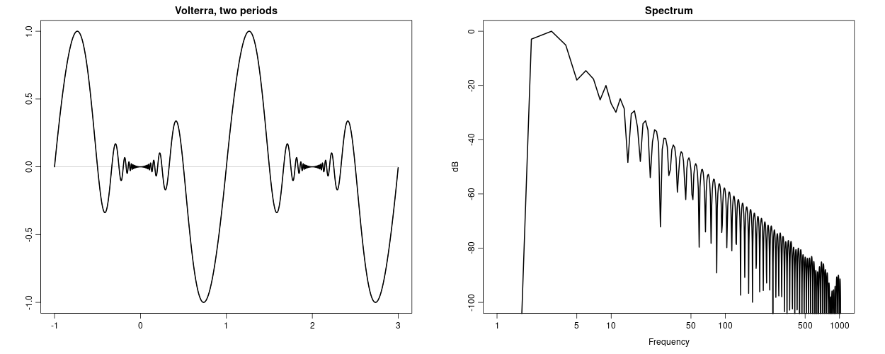
Note sequence using the Volterra waveform.

Pathological octaves

void make_octaves(REAL *wt, int N, bool norm=true)

A spectrum with only octaves is used in the Shepard/Risset illusion, where the partials' amplitudes are given by a gaussian function. This is a different example: the infinitely differentiable, yet not analytic function $$ f(x) = \sum_{k=1}^{\infty} {\exp(-\sqrt{2^k}) \cos (2^k x) }. $$ What is true of an infinite series does not necessarily hold for a finite summation. As usual, as long as aliasing is avoided this one sounds pretty much as expected.

Glissando with the octave waveform.

Darboux nowhere differentiable

void make_darboux(REAL *wt, int N, bool norm=true)

Yet another real analysis example: a nowhere differentiable function—if you have the patience to add an infinite number of partials. This one is actually bandlimited, but contains some very high partials. (The highest partial covers one period over at least four samples in the table.) $$w_{t}=\sum_{k=1}^{p}\frac{\cos(2\pi k!t)}{k!}$$ For best results, use a long wavetable.

Glissando using the Darboux waveform.

The Darboux function is an example of lacunary trigonometric series, as are the following functions.

Sparse spectrum

void make_sparse(REAL *wt, int N, int P=55, bool one_over_k=true)

Sparse spectrum. As the fundamental frequency becomes sufficiently low the perceived pitch may jump up to a higher partial.

Sparse spectra have widely spaced partials. The waveform generated by make_sparse is built from partials at the triangular numbers $T_k = 1,3,6,10,15, ...,$ with decaying amplitude. If the parameter one_over_k is true the amplitudes are $a_k = 1/k,$ otherwise the amplitude is inversely proportional to the frequency, that is, $a_k = 1/T_k.$ This waveform has a peculiar fractal appearance.

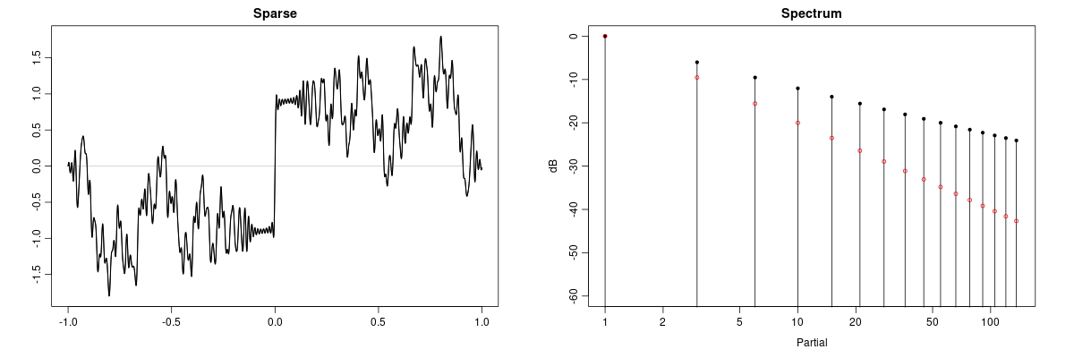
Sparse waveform generated with $a_k=1/k$ and spectrum with both spectral slopes shown. The red dots correspond to $a_k = 1/T_k.$

void make_prime(REAL *wt, int sz, int p=10, bool norm=true)

Selecting only prime number partials likewise creates a sparse spectrum with similar character to the one generated from partials at triangular numbers.

Prime number partials.

~~~

Home

Research

Music

Video

Programming

Text

Drawings

Links

About me

Download