Synchronization of chaotic modules

Chaotic oscillators

In the world of modular synthesizers, most analog oscillators or LFOs all seem to be minor variations on the same design. They have more or less the same inputs and they output more or less the same set of waveforms. But oscillators can be so much more. There are many dynamic systems that are capable of periodic oscillations. Nonlinear dynamic systems may also become chaotic.

Chaotic signals are noisy and irregular. But if the dynamic system has parameters that can be varied, then its dynamics will depend on the position in the parameter space and one may see various kinds of bifurcations from fixed points to cycles, period doublings and chaos, and perhaps quasi-periodic orbits. When the orbits are periodic, their period may be influenced by tuning some parameters, but doing so the waveshape typically also changes. Chaotic modules usually do not have a simple control voltage input allowing for precision tuning comparable to the V/octave standard of ordinary VCOs.

The practical solution, if one wants to have more control over a chaotic system, is to modulate some of its parameters. This is one of the techniques used in chaos control. By sending a periodic signal to the chaotic system and modulating any of its parameters, one can make the system lock in to the forcing period. A chaotic system may also synchronize to another chaotic system, depending on the strength of the coupling and the nature of the two chaotic systems. In the case of periodic forcing, the slave system may lock to periods which are related by some rational number to the period of the master system. But the driven system may also fail to synchronize to the forcing signal. What happens depends on a number of factors, such as the frequency, amplitude and waveform of the driving signal.

A slow and a fast system

Dynamic systems operate on particular characteristic time scales. This can be demonstrated with two Eurorack modules, one of which typically oscillates in the sub-audio range, whereas the other one spans a much broader range, reaching high audio frequencies.

The Snazzy FX Chaos Brother has two knobs that tune the system's parameters: one is called chaos and the other one speed. Their effect on the dynamics are almost self-explanatory; when “chaos” is turned down to zero, “speed” controls the rate of the periodic oscillation, and when the chaos knob is turned up, the system at some point becomes chaotic. There is also one cv input which can be used to synchronize the system and make it oscillate on a much broader range of frequencies than it would do without input.

The Chaos Brother has two outputs labeled X and Y, as well as two other outputs that need not concern us now. If the X and Y signals are plotted each on its own axis, one gets a picture of the attractor of the system. The X signal is faster and bumpier than Y.

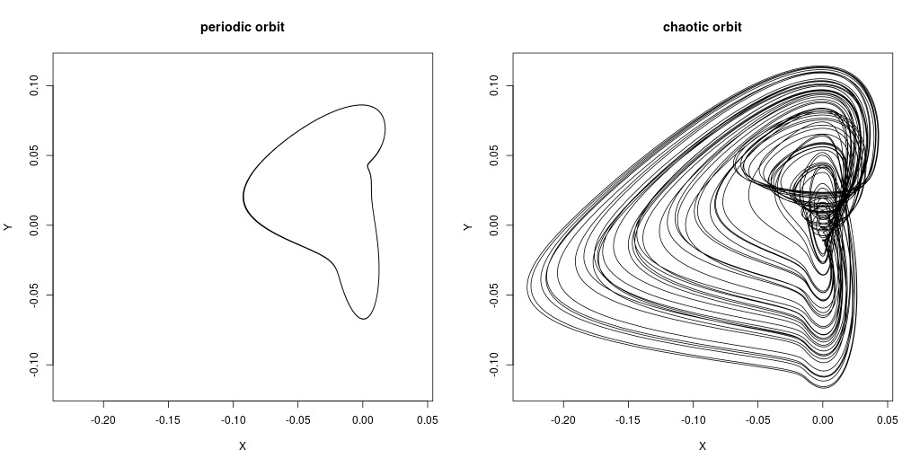
A limit cycle as seen on the left is just a periodic waveform. The other attractor is apparently chaotic.

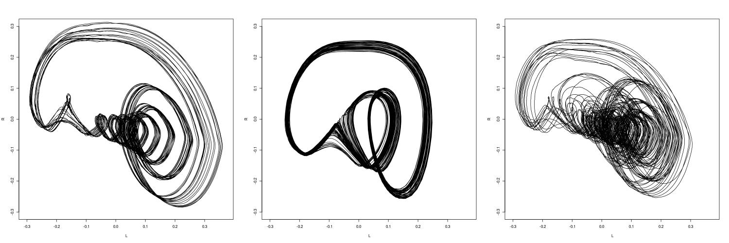
Elby Design's Chaotica (derived from the Jerkster, designed by Ian Fritz) is a much more complex module, which is described as a third order system with four nonlinear elements. It has four main parameters each with cv input: these are called rate, damping, offset and gain. There is also a knob for a parameter called NL drive and two switches, one for “wild” or “tame” and another for 1 or 2 “eyes”. Then there is an input labeled “reset - inhibit”, which does just that. There are three outputs labeled X, Y and Z. In the following plots, the X and Y signals have been used. It is very easy to find periodic orbits with Chaotica, but the attractors below display chaotic orbits.

Synchronization

We now return to the Chaos Brother and look at how it responds to an incoming periodic cv signal.

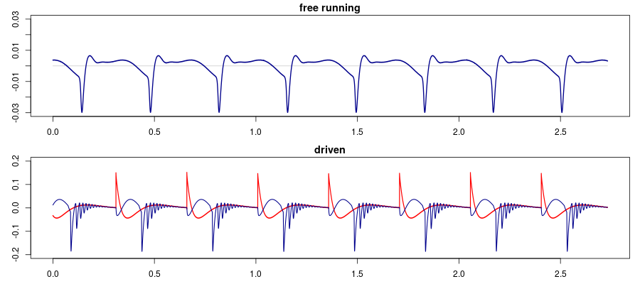
In the top plot, the X output is shown. The speed knob is at minimum and the chaos knob at noon, and there is no cv input. There is a periodic oscillation at slightly less than 3 Hz.

The bottom plot shows what happens when a sawtooth waveform (red) is fed to the cv input. The sawtooth is also slightly below 3 Hz and looks more like a spike, but that is perhaps due to its very low frequency not being well captured in the recording. Apart from having the same overall period as the driving sawtooth, the blue curve which comes from the X output also has some rapid wiggles, and its amplitude is significantly greater when receiving cv input.

In this case, the driving signal happens to have almost the same period as the free-running system, so when fed the sawtooth it has no problem locking in to it.

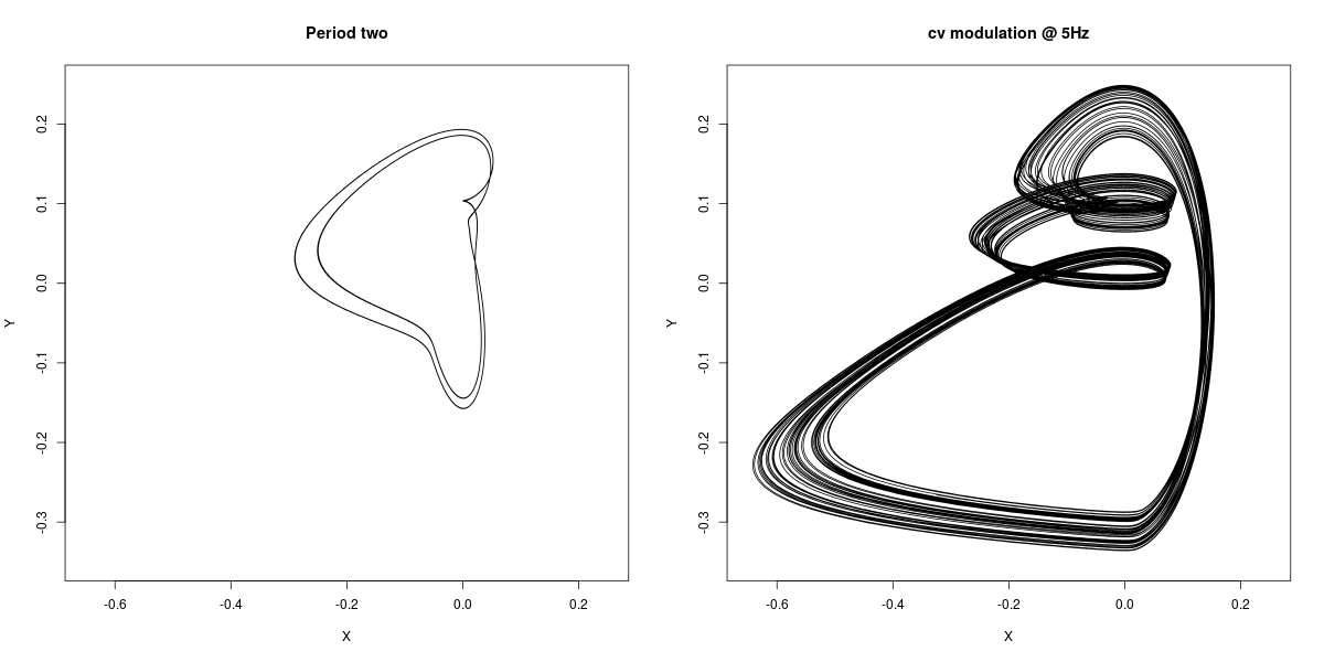
Here is a phase plot of the system with and without forcing. To the left the system runs without input, and it has now entered a period two orbit. In this example Chaos is at noon and Speed around 9 o'clock. The right panel shows the system forced by a sawtooth wave at approximately 5 Hz and the cv attenuator set half-ways. We see what appears to be a chaotic attractor, again with substantially larger amplitude than in the unforced system.

Next, let us try a faster forcing signal. Now the forcing sawtooth's fundamental frequency is 75 Hz, which is way above the chaos brother's inherent range.

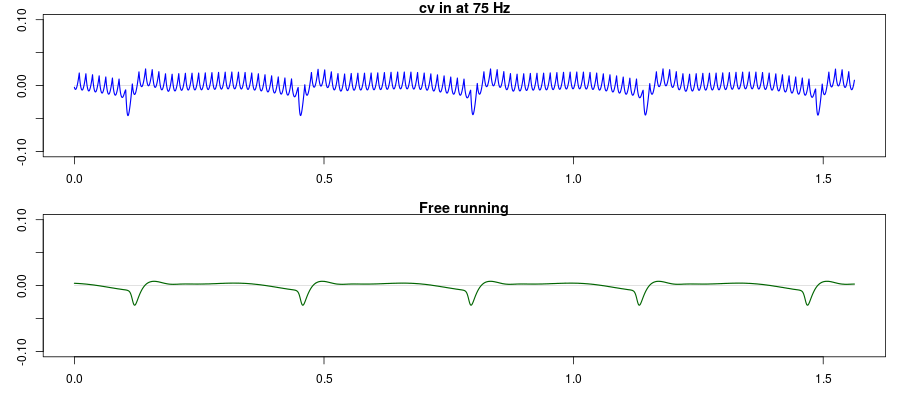
The top plot shows how the X variable responds to this fast sawtooth. Its rapid wiggles lock tightly to the incoming sawtooth, but superimposed there are regular dips on its own natural frequency, as can be seen in the bottom plot where there is no cv input.

The Y variable also responds to cv modulation, but since it is a slower variable its response is less pronounced.

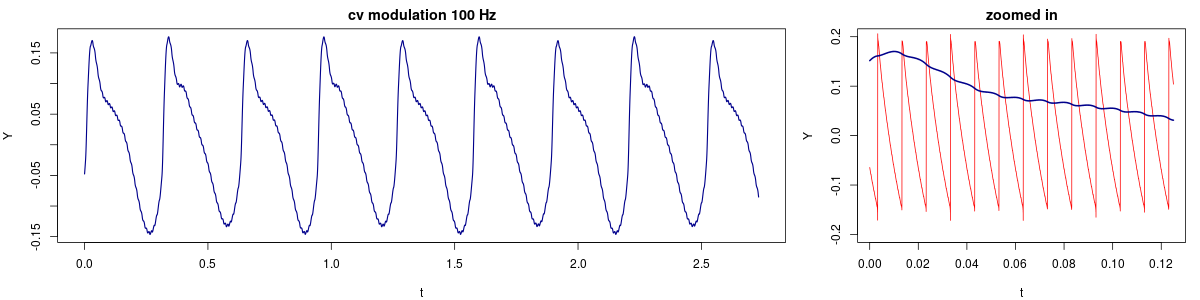
Here the sawtooth's frequency is 100 Hz. Some extremely small wiggles can be observed on the Y waveform, and zooming in it can be seen that the wiggles are locked to the sawtooth modulator.

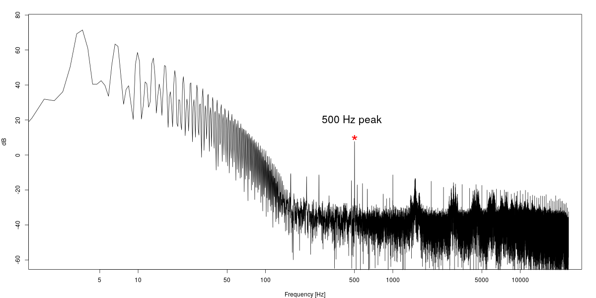
Finally, we break all speed records and set the forcing sawtooth to 500 Hz. With really fast forcing the time scales of the two systems are so different that they are difficult to display simultaneously, but we'll try.

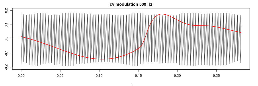
Apparently the slow Y variable (red curve) doesn't react at all to the incoming 500 Hz sawtooth cv modulation (in black). We will have to look at Y's spectrum for the forcing signal to be detectable. Even then it turns out to be about 60 dB weaker than the peak around 3 Hz which is the natural frequency of the system.

Further enquiry

We have treated the module as a black box, but its maker or someone better versed in electronics would be able to write down the differential equations that are at work here. With a simplified set of equations and parameters corresponding to the knobs on the module, one could easily simulate the system and map out its behaviour in the parameter space by bifurcation diagrams. If one had cv inputs instead of knobs to control the two parameters this experiment could be carried out with the module and a precision constant voltage generator.

We have only used periodic sawtooth waveforms as the forcing signal, but different waveshapes may cause different behaviour. The forcing signal's amplitude has a clear effect on the dynamics. Weak signals have little or no effect, whereas strong forcing signals more easily make the slaving system lock in to the master's periodicity. Instead of using a periodic signal, we could have used a chaotic forcing signal, although it would have been harder to analyse whether synchronization happens or not.

We have focused on the Chaos Brother which acts like an LFO. Chaotica, on the other hand, spans a broader range but is typically used in the audio range, and can be thought of as a VCO. As we have just seen, too rapid a forcing signal will not wake a slow system from its lethargy. But might it not nevertheless be interesting to connect these two chaotic modules together? Of course any patching could be worth trying, but let us take a more theoretical view for a moment.

Slow-fast systems

We have a suspicion, based on a small number of experimental observations, that a system can most easily synchronize to another if its internal or "natural" frequency is not too different from that of the forcing signal. Therefore connecting one of the fast system's (say, Chaotica's) outputs to the cv in on the slow system will not have a great deal of effect as long as the fast system oscillates rapidly. Conversely, we may connect one of the slow system's outputs to a cv input in the fast system. Now, this is different, because these slow parameter variations cause changes in the fast system. The pitch may fluctuate and the waveform may vary, and the fast system may alternate between chaotic and periodic states.

In the dynamic systems litterature, this is known as slow-fast systems. In general, they are described by the equations $$ \dot{x} = f(x,y) $$ $$ \dot{y} = \varepsilon g(x,y) $$ in which $\varepsilon$ is a small number, and both $x$ and $y$ may be vectors. The small $\varepsilon$ in the second equation ensures that the time derivative takes on small values, so this is the slow subsystem.

Often slow-fast systems are studied with one-directional coupling as we did above, which means that one system drives the other. If the fast subsystem drives the slow system, the fast orbit $x(t)$ will travel around its attractor many times while the slow orbit $y(t)$ only covers a small segment of its attractor. Hence the fast orbit will appear as noise to the slow system and it may be adequately approximated as its average value $\left\langle x(t)\right\rangle$ plus a noise term $\xi(t)$ with expected value 0, that describes fluctuations around the mean. If the noise term is sufficiently weak it may be ignored altogether, which leaves the slow system with a constant term as input and the second equation becomes $\dot{y}=\varepsilon g(\left\langle x\right\rangle ,y)$.

Now let us consider the opposite direction of coupling, so that the fast system is driven by the slow system. This means that the fast system will have slowly drifting parameter values. In the limit, with a sufficiently large separation of time scales, the fast dynamics can be approximated over finite time segments by the dynamics of the fast subsystem with constant parameters.

In case of mutual coupling, we may still expect the fast subsystem to contribute small fluctuations to the slow system, and the slow system causing a parameter drift in the fast system. However, if the fast system moves into parameter regions with qualitatively different behaviour, i.e., it bifurcates to another type of orbit, the average may change and the fluctuation term will have a different distribution. This in turn influences the slow dynamics.

Peeking into the blackbox

Although one has no idea of which equations describe a dynamic system, one could make an educated guess. Typically, when doing time series analysis of unknown, possibly chaotic systems, one has access only to a single variable which can be analysed by means of time delay coordinates. Here we are lucky, because we have two or three outputs from a module, which presumably are actual phase space variables.

Ordinary differential equations must be nonlinear and have at least three dimensions for them to be chaotic. The requirement of three dimensions for chaos is known as the Poincaré-Bendixon theorem. There are two ways to express a system of ODEs. Suppose we have a three-dimensional system. The most common way to express this system is as three coupled equations: $$\dot{x} = f_1(x,y,z) $$ $$\dot{y} = f_2(x,y,z) $$ $$\dot{z} = f_3(x,y,z). $$ Another way of expressing a three-dimensional system is as a jerk equation, or a third order differential equation with jerk (third derivative) on the left hand side: $$\dddot{x} = f(\ddot{x}, \dot{x}, x)$$ When this system is expanded to three first order equations, one makes the substitutions $\dot{x} \to y$ and $\ddot{x} \to z$, which leads to the system $$ \dot{x} = y $$ $$ \dot{y} = z $$ $$ \dot{z} = f(x,y,z). $$ Here we notice that $y$ is the derivative of $x$, and $z$ is the derivative of $y$. The frequency domain equivalent of derivation is high pass filtering. Hence one would expect $y(t)$ to be a faster and brighter signal than $x(t)$, and similarly $z(t)$ should be faster and brighter than $y(t)$.

Working in the opposite direction with two or three outputs recorded from a module, we could try differentiating each signal to see if it then becomes identical to one of the other signals.

Practical ideas for modular patches

When connecting a slow and a fast system, one can increase the influence of the fast system on the slow by emphasizing its slow fluctuations. This can be done with a lowpass filter or by other means that reduce the rate of fluctuations. A sub-octave generator can also be useful.

Going from the slow to the fast system, the slow modulation will cause continuously sliding parameter values if it is directly connected to the fast system. If this is unwanted, these signals can be passed through a quantizer or a sample and hold circuit.

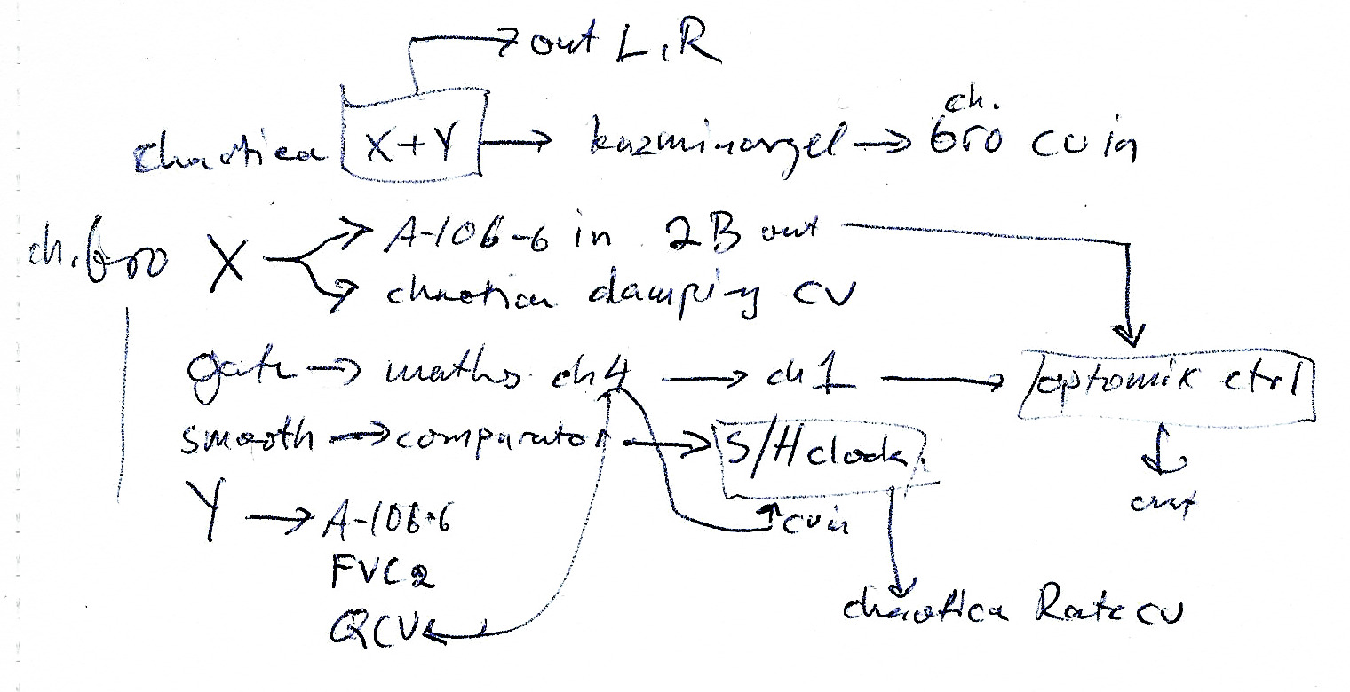
Here is a fully auto-generative patch with a few more modules, but the basic idea is to set up a cross-modulation between the fast and the slow chaotic modules. The audio output comes from chaotica's X and Y outputs as well as a bandpass filter fed with Chaos Brother's X and its cutoff modulated by its Y output and the time-variable Q-factor modulated by a slew-limited version of the gate output. The smooth output goes to a comparator which sends clock signals to a S/H, which samples the slew-limited gate. The S/H output goes into Chaotica's Rate cv input, which creates the seemingly random sequence of pitches. Finally, the Damping cv input receives the Chaos Brother's X signal.

The first sound example consists of two parts whose only difference is that two parameters of Chaotica are different. This difference is enough to alter the dynamics completely, also in the slow rhythmic pattern. The second part begins at 32 seconds. Nothing is touched while the patch runs.