Variations of Frequency Modulation

Take a vibrato and increase its rate to audio frequencies. This is the basic idea of frequency modulation, a synthesis technique widely used since Chowning stumbled upon it in the 1960's. Several extensions and variations of the original two-oscillator FM algorithm have been proposed, many of them implemented in hardware synthesizers, as software, or described in papers. But there is scope for further experimentation.
There are lots of tutorials and introductions that cover FM synthesis from a theoretic as well as a sound design point of view (see references below). Here I will focus on some less well known aspects of FM from a theoretical perspective, assuming the elements to be known. After a brief overview I will discuss:
feedback FM and chaos,
some other ways of using feedback,
FM with a linear ramp modulator,
and exponential FM.
Basic operator architectures
The most basic FM setup uses two oscillators where the first modulates the frequency of the second. The frequency of the second oscillator is called the carrier frequency, $f_c$, and the frequency of the first oscillator is the modulation frequency, $f_m$. A modulation index determines the size of the deviation around the carrier frequency.
Frequency being the rate of change of the phase, FM is very closely related to phase modulation. In fact the distinction is often hard to make, so I will not be pedantic about the difference unless it really matters.
Some of the most common arrangements of FM oscillators are the following, roughly ordered by increasing complexity.
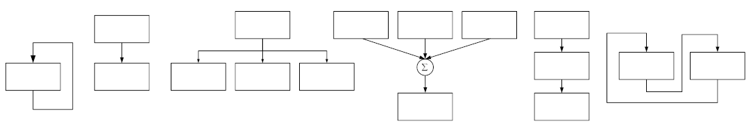
From left to right:
- Feedback FM
- Classic two oscillator FM
- One oscillator modulating several carriers
- Many modulators summed and modulating one carrier
- Cascaded or stacked FM
- Cross-coupling
Feedback FM usually refers to a single oscillator whose output is fed back and added to the current phase (see below for a closer analysis).
Classic FM with two oscillators may be extended by splitting the modulator and feeding several carriers with it. This can be a convenient way of introducing formants.
When two or more modulators are summed before modulating the carrier frequency complicated intermodulation occurs. This type of intermodulation happens even in ordinary two oscillator FM if the modulator is a complex harmonic tone instead of a single sinusoid.
In cascaded FM one oscillator modulates the second, which in turn modulates a third oscillator, and the chain of oscillators could be made even longer. Since the signal coming out of the second oscillator is already likely to have a few prominent partials the effect will be similar to having a vast array of separate modulators connected to one single carrier.
Cross-coupling is less well known, but can be easily achieved with a pair of analog oscillators by patching an audio output of one oscillator into the pitch cv input of the second oscillator, and vice versa. Nor is it difficult to cross-couple digital oscillators (except in environments that use buffer processing that prohibits feedback from the previous output sample), but the results can be hard to predict.
For any given FM operator structure the ratio of modulator to carrier frequencies (c:m ratio) and the modulation index are the parameters that shape the sound. In practical use of FM the parameters are usually tuned by hand, perhaps guided by some heuristics and received wisdom. Another approach is to search the parameter space by genetic or other algorithms in an effort to find close matches to specific target sounds.
The FM equation and spectrum
For reference, classic FM (or PM, phase modulation) is obtained by adding a modulator signal $\sin (\omega_m n$) to the carrier $\omega_c$ as the argument of a sine function, $$ x_n = A \sin(\omega_c n + I \sin(\omega_m n)), $$
where $I$ is the modulation index and the radian frequencies $\omega$ are related to frequency $f$ by $\omega = 2\pi f/f_s$ with sampling rate $f_s$ Hz. Frequency modulation produces a spectrum with partials at $\omega_c \pm k \omega_m$, in other words, symmetrically spread around the carrier frequency by integer multiples of the modulator frequency. The relation $$ \sin(\omega_c t + I \sin \omega t) = \sum_{k=-\infty}^{\infty}{J_k(I) \sin(\omega_c t + k\omega_m t) } $$ shows how to calculate the amplitude of each partial of the FM spectrum using the special functions $J_k(I)$ which are ordinary Bessel functions of the first kind, of integer order $k$ and with the modulation index $I$ as their argument.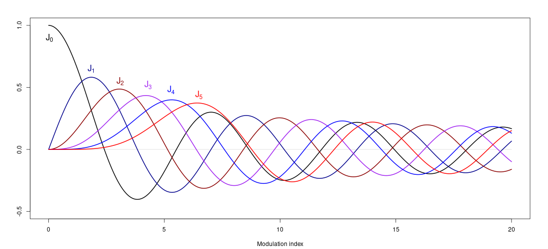
Bessel functions of order 0 to 5. Each Bessel function oscillates and slowly decays, and functions of increasing order reach their maximum at a higher modulation index.
What makes the calculation of the spectrum somewhat intricate is the fact that these Bessel functions can be both positive and negative, and those of negative order are defined by $J_{-k} = (-1)^kJ_k$. Negative frequencies must be taken into account, and all of this leads to possible phase cancellations when positive and negative frequencies coincide. In practice, however, FM can be used quite intuitively by trying out different operator structures and values for the parameters. In the early days of FM some people probably obsessed more about calculating the spectrum before composing with it.
Complex modulators
The case of FM with a complex modulating signal is particularly interesting. By a 'complex' modulator we mean one that is the sum of more than one sinusoid. Let's say there are two sinusoidal modulating signals, so the synthesis equation becomes $$ x_n = A \sin (\omega_c n + I_1 \sin(\omega_{m1} n) + I_2 \sin(\omega_{m2} n)) $$ with modulation frequencies $\omega_{m1,2}$ and modulation indices $I_{1,2}$. For an intuitive understanding, a useful way to think about this is to regard the outermost sine function as some kind of waveshaper, where the signals fed into it are mixed and squashed. In waveshaping of two periodic signals there will be intermodulation products at multiples of the sums and differences of the two frequencies. This is exactly what happens in FM with complex modulating signals. With two modulators, the spectrum will have partials at $ \omega_c \pm i \omega_{m1} \pm j \omega_{m2} $ for all integers i and j. The spectrum easily becomes extremely dense, although the amplitude of each partial scales as $$ \omega_c \pm i \omega_{m1} \pm k \omega_{m2} \longleftrightarrow J_i (I_1) J_k (I_2) $$ which becomes relatively small for most of the partials since the Bessel functions are bounded by 1 in magnitude. The case of three or more sinusoidal modulators is handled analogously. A derivation of the equations can be found in a classic paper by Le Brun (1977) and some practical sound design ideas for strings and piano sounds are provided in another classic paper by Schottstaedt (1977).
Side note on "thru zero" FM
Frequency modulation can be done with analog oscillators, although the fine tuning of the c:m ratio and the stability required for precise sound design benefits from digital implementations. In the analog world there are basically two kinds of FM: exponential (see below) and linear. Furthermore, analog oscillators have two variants of linear FM. One is notoriously known as thru zero FM, and appears to be surrounded by an aura of mystique. What it actually means is that the modulator signal is exactly what we would expect, a bipolar signal that passes through zero!
It is the other kind of FM that begs for an explanation. In non-thru-zero or positive linear FM the modulator signal is restricted to be non-negative. For a sinusoidal or triangle modulator wave this half-wave rectification deforms the waveshape and adds a series of partials, which produces a denser spectrum with more prominent high partials.
Feedback FM considered as an iterated map
Classic two-oscillator FM arguably suffers from a shortcoming. An easily recognised sonic signature is revealed when the modulation index is varied. The Bessel functions' undulating shape makes the spectral profile vary in ways that are untypical of acoustic instruments. In contrast, the advantage of feedback FM is that its spectral profile changes smoothly and predictably with the modulation index.
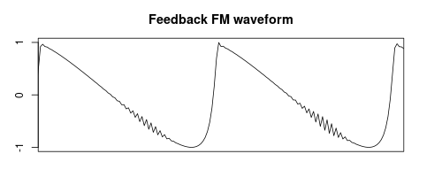
Feedback FM as described by the equation $$ x_n = \cos(\omega n + \beta x_{n-1}) $$ is restricted to harmonic tones, at least as long as the modulation index $\beta$ is kept within a certain limit. Pushed beyond that limit first a certain disturbance enters and finally the tone turns into chaotic noise. Aliasing is a concern at high frequencies and more so with increasing modulation index. At $\beta=0$ the output is just a sinusoid, but as the modulation index increases to about $\beta=1$ the waveform approaches an harmonically rich sawtooth shape.
Sound example: Feedback FM with modulation index rising from 0 to 5.
As Norio Tomisawa noticed in his patent description, at a certain point as the modulation index increases a spurious fast oscillation is superposed on the waveform. This hunting phenomenon, as it is referred to in the patent, consists of an oscillation at the Nyquist frequency in parts of the wavecycle. It is best understood from the perspective of iterated maps. Hence we write the feedback FM equation as the iterated 2D map $$ \begin{align} \theta_{n+1} &= \theta_n + \omega \\ x_{n+1} &= \cos(\theta_n + \beta x_n) \end{align} $$ with initial conditions $\theta_0$ and $x_0$.
An oscillation at the Nyquist frequency is a period two solution in the context of iterated maps. Period two orbits usually follow a period one orbit as part of a period doubling bifurction sequence. Here, however, the 2D system already oscillates at the radian frequency $\omega$, so one may be led to believe that the hunting does not appear out of a common period doubling bifurcation.
In order to better understand what goes on we simplify the system by setting the frequency to zero. Although that is not very useful for sound synthesis it makes it easier to analyse the system's dynamics. Now there is a constant phase term $\theta_0$ that we will get rid of by setting it to zero. Then the equation reduces to the one-dimensional map $$ x_{n+1} = \cos(\beta x_n) $$ which we can run at various values of $\beta$ to see what happens. An initial value $x_0$ must be chosen, and it should not be one of the fixed points $x^* = \cos(\beta x^*)$, so we will start the system from $x_0 = 0$ and omit the initial transient of the first few iterations from the plot.
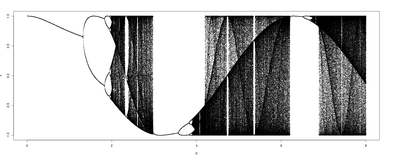
Bifurcation plot of feedback FM for $0 < \beta < 8$ and $\omega=0$.
As the bifurcation plot shows the first period two orbit sets in at $\beta \approx 1.319$. In fact the hunting phenomenon begins to appear already at slightly lower modulation indices. A possible explanation is that these period two oscillations are transients that occur while the map approaches its fixed point. These transients are decaying oscillations that become more long-lived as the bifurcation point is approached. When the feedback oscillator runs at higher frequencies $\omega$ the hunting phenomenon also sets in for lower modulation indices.
Tomisawa's patent suggests a simple solution to squelch the spurious oscillations, or at least to be able to increase the modulation index to a slightly higher level before they set in. The quick fix is to insert a simple two point average lowpass filter $y_n = \frac{1}{2} (x_n + x_{n-1}) $ in the feedback path.
Sound example: Feedback FM with modulation index rising from 0 to 5 as in the previous
example, but this time with a two point average filter in the feedback loop.
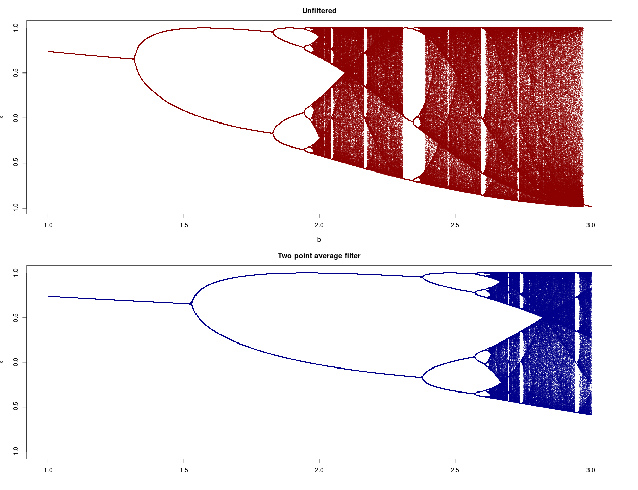
Comparing the two methods shows that the period doubling sequence is shifted towards a higher modulation index when the two-point average method is used, and also the parametric range of the stable period two orbit becomes significantly enlarged.
The two-point average lowpass filter introduces one new state variable to the system, which now becomes $$ x_{n+1} = \cos(\omega n + \frac{\beta}{2} (x_n + x_{n-1})). $$ Higher order lowpass filters, or really any filter, can be inserted in the feedback path. This is a field open to all kinds of experimentation.
Sound example: Feedback FM, again with modulation index rising from 0 to 5. A third order allpass filter
followed by a one-pole lowpass filter inserted in the feedback path distinctly colours the sound.
The bifurcation plots above show what happens in feedback FM when the frequency is zero. There is a period doubling cascade followed by chaos, then there are more periodic windows and chaos as the modulation index increases further. The analysis could be extended to positive carrier frequencies, but the conclusion is that feedback FM should be understood as an iterated nonlinear map. A suitable name for this map might be the cosine map, but for some reason almost all papers instead refer to the sine map. Anyway, the sine and cosine maps are related by a simple change of variables, and their dynamics closely resemble that of their much better known relative, the logistic map.
Other types of feedback
Feedback amplitude modulation (FBAM) has been proposed as a simple synthesis technique. One of its forms is $$ y_{n+1} = \cos (\omega n) (1 + \beta y_n). $$ Insofar as there is such a thing as feedback ring modulation its equation would look similar, except that the constant term 1 in the paranthesis is dropped, so when $y_n = 0$ the fun is over because the oscillator would stop oscillating at that point.
In fact, the feedback FM equation can be manipulated in an interesting way to show that it too is related to some kind of amplitude modulation. First, use the formula $\cos(a + b) = \cos a \cos b - \sin a \sin b$ to rewrite the feedback FM equation $$ x_{n+1} = \cos (\theta_n + \beta x_n) $$ as follows: $$ x_{n+1} = \cos (\theta_n) \cos (\beta x_n) - \sin(\theta_n) \sin (\beta x_n). $$ This expression can be put more succinctly as the real part $x = \Re (z)$ of a complex variable $z_n = e^{i(\beta x_n - \theta_n)}$. Then the feedback FM equation may be written as the complex multiplication $$ z_{n+1} = e^{-i \theta_n} e^{i \beta \Re (z_n) }. $$
Loopback FM is a recently introduced variant of FM in which the oscillator's output is used to modulate the frequency instead of the phase of the oscillator. Its equation $$ z_{n+1} = z_n e^{i \omega (1 + B \Re (z_n))} $$ is not too dissimilar from FBAM or the complex formulation of feedback FM. The system is started from an initial condition $|z_0| = 1$ and the modulation index should be restricted to the range $-1 < B < 1$. In loopback FM the pitch decreases as the magnitude of the modulation index increases, until at $|B| = 1$ the oscillator slows down to a halt. In many situations this pitch inflection is inconvenient, but as Hsu and Smyth suggest it can be useful in the synthesis of percussion sounds, and probably in a few other situations as well. In any case they have derived a relation between the modulation index and the resulting pitch that enables separate control of both modulation amount and pitch.
Sound example: Loopback FM with modulation index rising from 0 to 1 over the sound's duration.
Yet another type of feedback FM expressed in complex variables should be mentioned. Dan Slater describes the cross-coupled system $$ u_{n+1} = u_n e^{-i(k_1 \Re (v_n) + \omega_1)} \\ v_{n+1} = v_n e^{-i(k_2 \Re (u_n) + \omega_2)} $$ of two complex exponential oscillators that produce chaotic FM. Again, notice the similarity with loopback FM. In this cross-coupled system the pitch also varies as a function of the modulation indices. Because of its perfect symmetry it makes no sense to call one of the variables the carrier and the other the modulator; they both modulate each other with amounts given by $k_1$ and $k_2.$
Sound example: Slater's chaotic FM with constant frequencies $\omega_i$ and time varying modulation indices.
Notice the staircase type of jumps in pitch in the beginning even though both modulation indices vary smoothly.
The noisy part at the end is where chaos sets in.
FM with linear ramp modulator
When analogue oscillators are used for FM any available waveform can be a modulator or a carrier. Waveforms rich in overtones generally produce very dense spectra and possibly harsh sounds. In digital implementations aliasing is a concern. Bandlimited waveforms should be used, yet oversampling might be called for. Instead of that proven method we will consider another idea which is not new; it is a special case of a technique introduced by Maurice Rozenberg under the name of linear sweep synthesis.
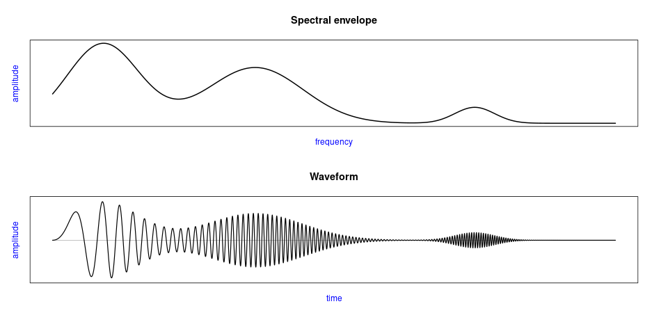
A spectral envelope (top) is applied to the amplitude of a sinusoid with linearly increasing frequency (bottom). This swept and amplitude modulated sinusoid is periodically repeated to create the linear sweep signal.
Take a linear ramp as the modulator waveform. While the ramp goes up the oscillator's phase increases at a rate given by the sum of the carrier frequency and the ramp. In effect this is a naïvely implemented sawtooth wave with all of its aliasing issues. Now, instead of creating a bandlimited sawtooth, suppose we rapidly fade out the output of the carrier oscillator exactly at the modulator's discontinuity. This is similar to applying the spectral envelope in linear sweep synthesis, or windowing signals in pitch synchronous granular synthesis. Specifically, suppose we use a raised cosine window $$ w(t) = \frac{1 + \cos \omega_m t}{2} $$ which depends on the modulation frequency $\omega_m = 2\pi f_m.$ If the carrier signal is $\cos (\omega_c t),$ then amplitude modulation with $w(t)$ produces two sidebands at $\omega_c \pm \omega_m$ besides the carrier.
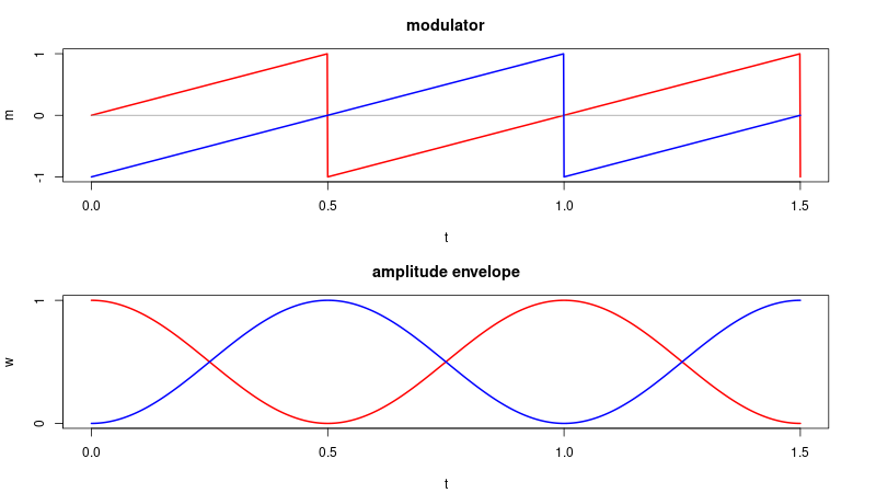
The two modulators offset by half a cycle and their corresponding amplitude functions.
To get rid of the amplitude modulation while keeping the linear ramp FM effect we need to introduce a second oscillator to fill in the gaps where the first oscillator is quiet, which we do by multiplying it with $1-w$ in order to have a constant amplitude when we sum the two oscillators. Thus, the modulators $$ \begin{align} m_1(t) &= 2f_mt + 1 \pmod 2 - 1 \\ m_2(t) &= 2f_mt \pmod 2 - 1 \end{align} $$ create the ramp waveforms in the complete system $$ x(t) = w(t) \cos(\omega_c t + I m_1(t)) + (1-w)(t) \cos(\omega_c t + I m_2(t)). $$ There is a noteworthy similarity with Shepard tones or, more properly, the Shepard-Risset glissando, the well-known auditory illusion of a constantly rising (or falling—or even both rising and falling) pitch. Shepard tones consist of sinusoids separated by octaves with their amplitudes defined as a function of the current frequency. Usually a gaussian function is taken as a spectral envelope to find the amplitude of each partial at each moment.
Practical implementations of Shepard tones would use a small number of oscillators with steadily rising frequency. As the frequency reaches the upper limit the amplitude simultaneously vanishes and at that point the oscillator is reset to its lowest frequency where the amplitude is also zero. The linear ramp FM oscillator as described above differs by using only two oscillators, and by having linear instead of exponential frequency modulation.
Sound example: Linear ramp FM with a slightly dropping carrier frequency, decreasing modulation
index and a decaying amplitude envelope produces this mellow bell sound.
The modulation index I plays a particular role in linear ramp FM. As defined, the ramp goes from -1 to 1 over one period. Consider the particular case $I=\pi.$ Since the modulator is now periodic in $2\pi$ we can add the carrier and modulator frequencies, so the output of the first oscillator is just a pure sinusoid at the new frequency $\Omega = \omega_c + \omega_m.$ The second oscillator's modulator being half a period out of phase, we have $$ x(t) = w \cos (\Omega t) + (1-w) \cos (\Omega t + \pi) $$ which reduces to $$ x(t) = \cos \omega_m t \cos \Omega t; $$ in other words, the pure ring modulation of two sinusoids with a spectrum containing nothing but the two partials at $\Omega \pm \omega_m,$ which evaluates to $\omega_c$ and $\omega_c + 2\omega_m.$ A similar thinning out of the spectrum occurs whenever $I$ is a multiple of $\pi.$
As we have seen, linear ramp FM is related to amplitude modulation. Turning up the modulation index increases the presence of side bands, but only up to a point where they begin to fade out and finally are reduced to those produced by ring modulation.
Sound example: Linear ramp FM with carrier 440 Hz, modulator 6 Hz and modulation index increasing from 0 to 13.
The slow modulation is heard as a warbling amplitude modulation. As predicted, the rising modulation index
is followed by a slight increase in pitch.
Instead of the ramp function we could take a pulse wave as modulator, which leads to the tremolo oscillator, as analysed in a previous paper.
Exponential FM
So far we have mostly considered examples of linear FM. In linear FM with a sinusoidal modulator the frequency deviation around the carrier is symmetric in Herz. Exponential FM is common in analog oscillators where a V/oct control voltage sets the oscillator's frequency. For each additional Volt on the oscillator's V/oct input the pitch rises one octave. If a symmetric waveform such as a sine or triangle is sent to the oscillator's input its pitch will vary exponentially in Hz, or linearly and symmetrically in semitones.
Sound example: Exponential FM with a triangle wave carrier from an analog oscillator (R*S NTO)
modulated by a sine wave from a self-oscillating filter. First the modulation amount increases,
then decreases back to nothing.
Exponential FM is not as well behaved as linear FM because the sideband frequencies depend not only on the carrier and modulator frequencies but also on the modulation index. For that reason it is probably most often used with constant parameters for inharmonic sounds such as bells.
The instantaneous frequency of exponential FM is $$ \omega_{IF}(t) = \omega_c B^{\cos \omega_m t} $$ with carrier frequency $\omega_c$, modulator frequency $\omega_m$ and modulation index $B > 0$. By integrating the instantaneous frequency we obtain the instantaneous phase $$ \phi(t) = \int_{0}^{t}{\omega_c B ^ {\cos \omega_m \tau} d\tau} $$ and the output signal $x(t) = \cos \phi(t).$ For the modulation index it makes sense to consider only $B \geq 1$ since the set of values $B^{\cos a}$ for $a \in [0,2\pi]$ is exactly the same as the set $(1/B)^{\cos a}.$ Substituting $\beta = \ln B \geq 0$ for the modulation index, the digital implementation of exponential FM would look something like this: $$ \begin{align} x_n &= \cos \phi_n \\ \phi_{n+1} &= \phi_n + \Omega_c e^{\beta \cos \theta_n} \\ \theta_{n+1} &= \theta_n + \Omega_m \end{align} $$ where $\Omega_m = \omega_m/f_s$ and $\Omega_c = \omega_c/f_s$.
Averaging the modulator over one cycle, $$ \frac{1}{2\pi} \int_{0}^{2\pi} e^{\beta \cos \theta} d\theta, $$ it turns out that the average is proportional to $e^\beta$, and so it is always positive. Therefore, when the modulator is added to the phase its positive offset from zero accumulates, which results in the frequency dependence on the modulation index in exponential FM.
Exponential PM
What sets exponential FM apart from linear FM is not only the exponential function, but also the multiplication with the carrier. This suggests we might instead try adding the exponential in the following way: $$ \begin{align} x_n &= \cos (\phi_n + \Omega_c e^{\beta \cos \theta_n}) \\ \phi_{n+1} &= \phi_n + \Omega_c \\ \theta_{n+1} &= \theta_n + \Omega_m. \end{align} $$ Thus we keep the exponential, but add the modulator to the phase of the carrier. What this really amounts to is the difference between frequency modulation (first version) and phase modulation (PM; second version). In a recent paper, Kasper Nielsen alludes to this idea without pursuing it further:
Like with Linear FM, it would be advantageous to use phase modulation to get an Exponential FM response. However, in practice this is difficult. Getting the instantaneous phase function would require integration of the above frequency function, but this does not have a closed-form solution. (Nielsen 2020)
We note that the practical numerical implementation poses no problem, despite the intractable evaluation of the integral.
Exponential FM and PM sound distinctly different. Most importantly, exponential PM does not suffer from the detuning and sidebands going haywire as the modulation index is changed.
Sound example: Exponential FM with increasing modulation $0 < \beta < 4$.
Sound example: Exponential PM with modulation $0 < \beta < 9$.
Both sound examples have $f_c = 660$ Hz and $f_m = 440$ Hz and a modulation index that increases linearly from 0. Due to the differences in scaling the modulation index values are not directly comparable between the two variants.
Waveshaping and ringmodulation
In exponential FM the exponential function acts like a waveshaper whose effects on a sinusoid input signal are easy to analyse. For that purpose it is illuminating to expand the exponential function into its Taylor series, $$ e^x = 1 + x + \frac{x^2}{2!} + \frac{x^3}{3!} + \cdots $$ from which we see that the sinusoidal modulator after passing the exponential waveshaper ends up as a sum $$ e^{\beta \cos \theta} = 1 + \beta \cos \theta + \frac {\beta^2}{2!} \cos^2 \theta + \cdots. $$ By expanding all the powers of the cosines such as $\cos^2 \theta = (1 + \cos 2\theta)/2$ into terms of the form $\cos k \theta$ we could derive the spectrum of the modulator. From there on we could, presumably, analyse the exponential FM spectrum in terms of the equation for linear FM with complex modulation signals. We refrain from doing so. Instead, it is interesting to observe what happens if we truncate the Taylor expansion after the second term: $$ e^{\beta \cos \theta} \approx 1 + \beta \cos \theta + \cdots $$ This term, when multiplied with the carrier, becomes $ \omega_c (1 + \beta \cos \theta) $, which is practically the same expression as we find for the instantaneous frequency in linear FM!
In digital synthesis one is aware of aliasing. Truncating the Taylor series after, say, the third of fourth term yields a reasonable approximation to the exponential function for low modulation indices, and at higher modulation index the approximated exponential grows less steeply and therefor introduces less high partials. This is at once an economic way of approximating the exponential and a simple aliasing reducing scheme. Furthermore, the approximating polynomial is just an arbitrary function, and we might experiment with waveshaping using other polynomials. For instance, a non-monotonous polynomial allows us to make the waveshaped FM have partials that slide up as well as down as the modulation index is increased.

Schematic of ring-modulated exponential FM.
In exponential FM, the dependency of the instantaneous frequency on the modulation index can be compensated for by lowering the modulation frequency as the modulation index increases. However, the higher partials will still spread out with an increasing modulation index, so in practice this is not a particularly satisfying solution. The problem, as we have noted, is due to the fact that the modulation signal averages to a positive number.
One way to get rid of this DC offset, which is hardly an original idea, is by ring modulation of the modulator with a sinusoid. Ring modulation introduces new partials in the modulator and the resulting spectrum is necessarily richer than that of ordinary exponential FM. In order to keep the resulting sound similar to that of ordinary exponential FM, the ring modulation frequency $f_r$ may be set equal to the carrier $f_c$, or to a simple ratio such as 2 or 1/2 to $f_m$. However, setting $f_r = f_m$ does not solve the DC offset problem. There can also be DC offsets in the output signal for some combinations of ratios. In general, any frequency could be assigned to the ring modulator, and the amount of ring modulation can be varied from none to full, which makes this hybrid technique ripe for further exploration.
Sound example: Three examples of exponential FM with ring modulation. In each example the modulation index
starts from 1.5 and decreases to zero. The $f_c : f_m : f_r$ ratios are (1:4:4), (3:4:8), and an inharmonic relationship
in the last example.
In contrast to linear FM of which there is no scarcity of information, exponential FM is not very much discussed outside the world of analog oscillators. If the theoretical derivation of sideband frequencies and their amplitudes is not precisely easy in linear FM, it apparently requires an even more heroic effort in exponential FM, as can be seen in a paper by B. Hutchins.
Other modulation techniques
There is also a thing called modified FM, $$ x_n = e^{iB \cos(\omega_m n)}\cos (\omega_c n), $$ which in some ways is similar to classic FM. Notably, modified FM differs by having its sideband amplitudes given by modified Bessel functions which are positive, whereas the ordinary Bessel functions of classic FM are bipolar with the complicated phase cancellations and reinforcements that may occur.
Many other nonlinear modulation techniques could be discussed here, since they are in some ways related to FM. Usually the distinction between frequency modulation and phase modulation is very hard to make, but, as we have seen with exponential modulation, sometimes it matters.
Synthesis by summation formulae is another group of nonlinear modulation techniques based on various expressions that have been discoverd to express infinite or finite sums of sinusoids in a closed form. Phase distortion and waveshaping are also related to FM. Some of the waveset distortion techniques introduced by Trevor Wishart may be combined with FM, such as waveset omission of cycles in the modulator. Recorded sounds can be frequency modulated by reading an interpolated delay line at variable rate. Nonlinear oscillators, often expressed as differential equations, can be combined with FM synthesis or other modulation techniques in interesting ways, but that is a topic for another day.
Further reading
John Chowning and David Bristow (1986). FM Theory & Applications. By Musicians for Musicians. Yamaha Music Foundation.
This book is a very accessible explanation of the maths behind FM with a few useful sound design ideas.
Bill Schottstaedt (1977). The Simulation of Natural Instrument Tones using Frequency Modulation with a Complex Modulating Wave.
Computer Music Journal, Vol. 1 No. 4, pp. 46-50.
Useful sound design ideas for piano and string sounds.
Mark Le Brun (1977). A Derivation of the Spectrum of FM with a Complex Modulating Wave. Computer Music Journal, Vol 1, No 4, pp. 51-52.
Lucid, concise, classic.
Bill Schottstaedt: An introduction to FM.
Good online reference for FM theory.
Daniel Beaufils: À propos de la synthèse F.M.
Mostly about the calculation of the FM spectrum, in French.
Alain Cassagnau: Analog-FM-Synth.
Another site in French about analog subtractive as well as digital FM synthesizers. There is also a book about FM.
John Chowning (1973). The Synthesis of Complex Audio Spectra by Means of Frequency Modulation.
Journal of the Audio Engineering Society, Vol 21, nr 7.
The classic paper that introduced FM as an audio synthesis technique.
Norio Tomisawa (1981). Tone Production Method for an Electronic Musical Instrument. US Patent 4,249,447.
Like so many patents this is not a very readable document, nevertheless
a standard reference for feedback FM.
Shah Abdullah Al Nahian, Zakir Hosen and Payer Ahmed (2019).
An Elementary Study of Chaotic Behaviors in 1-D Maps.
Journal of Applied Mathematics and Physics, 7:5, 1149-1173.
Concise tutorial on some key notions of chaos theory using the sine map as one of the examples.
Tamara Smyth and Jennifer S. Hsu (2019). Percussion Synthesis using
Loopback Frequency Modulation Oscillators. Proceedings of SMC 2019, Málaga, Spain.
Provides all the details to get started with loopback FM.
Tamara Smyth and Jennifer Hsu (2019). On Phase and Pitch in Loopback Frequency Modulation
with a Time-Varying Feedback Coefficient. 26th International Congress on Sound and Vibration.
Montreal.
After a clear explanation of concepts such as instantaneous frequency
and differences between phase and frequency modulation, the authors derive the formula for
the actual sounding frequency in loopback FM.
V. Lazzarini, J. Timoney, J. Kleimola, and V. Välimäki (2009).
Five
Variations on a Feedback Theme. Proc. of DAFx-09.
Not about FM, but a related class of modulation techniques called FBAM.
Risto Holopainen (2010). Self-organised
Sounds with a Tremolo Oscillator. Proc. of DAFx-10, Graz.
FM with a square or pulse wave modulator.
Andy Horner (2007). Evolution in Digital Audio Technology. In Miranda & Biles (eds): Evolutionary
Computer Music. Springer.
An overview of different synthesis techniques (including many variants of FM) and how to find sounds
that match specified target sounds by automated search in the parameter space using genetic algorithms.
Matthieu Macret, Philippe Pasquier, and Tamara Smyth (2012).
Automatic calibration
of modified fm synthesis to harmonic sounds using genetic algorithms.
Proc. of the 9th Sound and Music Computing Conf. Copenhagen, Denmark.
The authors find that the search for matching sounds with modified FM using a single modulator
and multiple carriers can be somewhat faster than using classic FM.
Maurice Rozenberg (1982). Linear Sweep Synthesis. Computer Music Journal, 6:3.
Largely overlooked, but interesting paper that generalises the idea of linear ramp FM.
Dan Slater (1998). Chaotic Sound Synthesis. Computer Music Journal, 22:2.
Nice discussion of analog modular synths and chaotic oscillators.
Bernard Hutchins (1975). The Frequency Modulation Spectrum of an Exponential Voltage-Controlled Oscillator.
J. Aud. Eng. Soc. 23:3.
An attempt to derive the spectrum of exponential FM as a function of
the modulation index. Also discusses some strategies for counteracting the pitch detunings caused
by varying the modulation index.
Kasper Nielsen (2020). Practical Linear and Exponential Frequency Modulation for Digital Music Synthesis. Proc. of DAFx, Vienna, Sept. 2020-21.
Compares linear and exponential FM and considers the detuning caused by the modulator's DC offset.© Risto Holopainen 2020